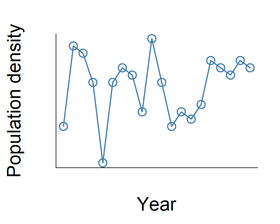
Recall: local population
Local population dynamics with no dispersal is driven by birth \(b\) and death \(d\) processes
\[
\frac{dN}{dt} = (b - d)N
\]
Once the population goes extinct, no chance to re-establish a new population
Immigration
Immigration can lead to a colonization into a new habitat
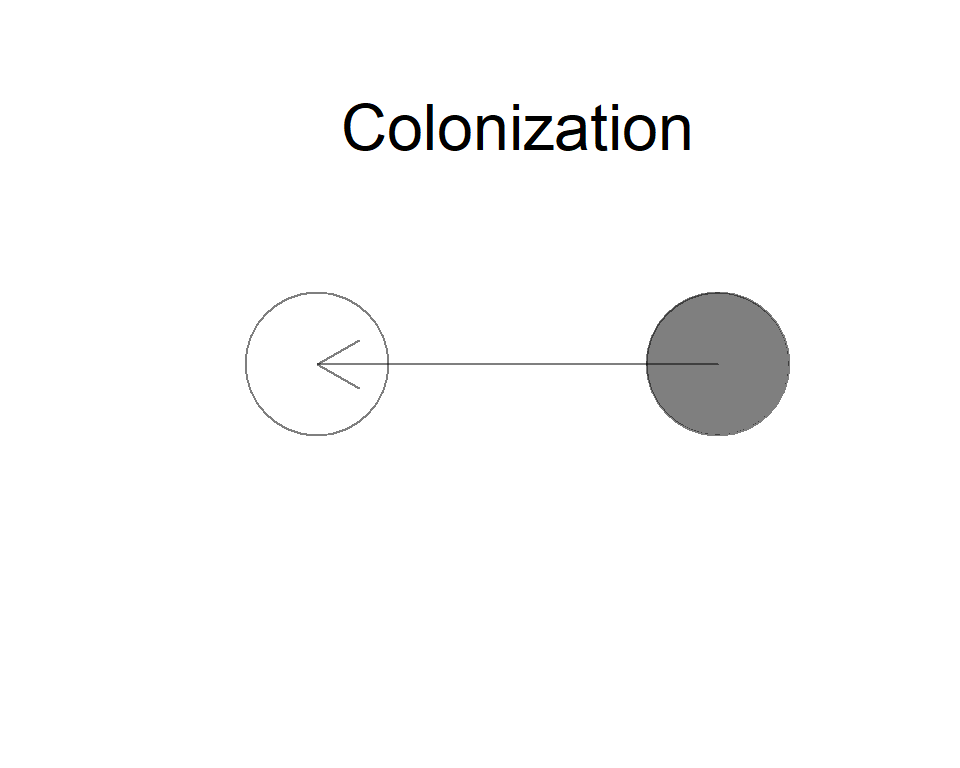
Colonization
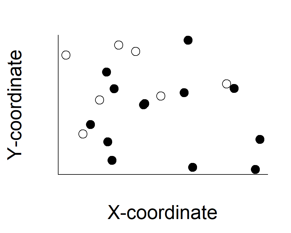
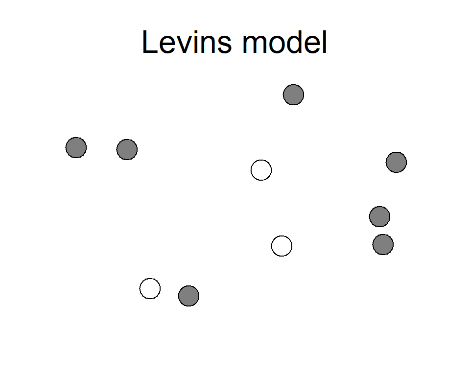
The Levins Metapopulation Model:
\[
\frac{dp}{dt} = mp(1-p) - ep
\]
The term \(mp(1-p)\) determines the rate of increase in occupancy
- immigrants come from occupied patches (\(p\))
- colonization occurs only at unoccupied patches
- multiply \(m\) to express random colonization
Extinction
The Levins Metapopulation Model:
\[
\frac{dp}{dt} = mp(1-p) - ep
\]
The term \(ep\) determines the rate of decrease in occupancy
- extinction occurs only at occupied patches (\(p\))
- multiply \(e\) to express random extinction
R exercise: colonization
Draw how colonization rate changes over \(p\)
Create \(p\) and \(m\) (set 1.0 for an example)
p <- seq(from = 0, to = 1, length = 100)
m <- 1
R exercise: colonization
Draw how colonization rate changes over \(p\)
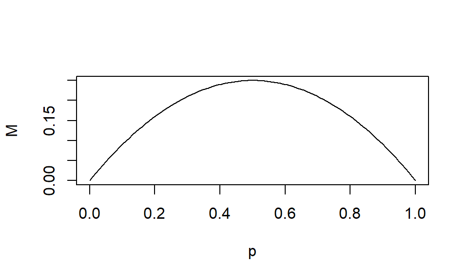
Plot the relationship b/w \(p\) and \(mp(1-p)\)
M <- m*p*(1-p)
plot(M ~ p, type = "l")
R exercise: colonization
Draw how colonization rate changes over \(p\)
Plot the relationship b/w \(p\) and \(mp(1-p)\)
M <- m*p*(1-p)
plot(M ~ p, type = "l")
R exercise: extinction
Draw how extinction rate changes over \(p\)
Create \(e\) (set 0.2 for an example)
R exercise: extinction
Draw how extinction rate changes over \(p\)
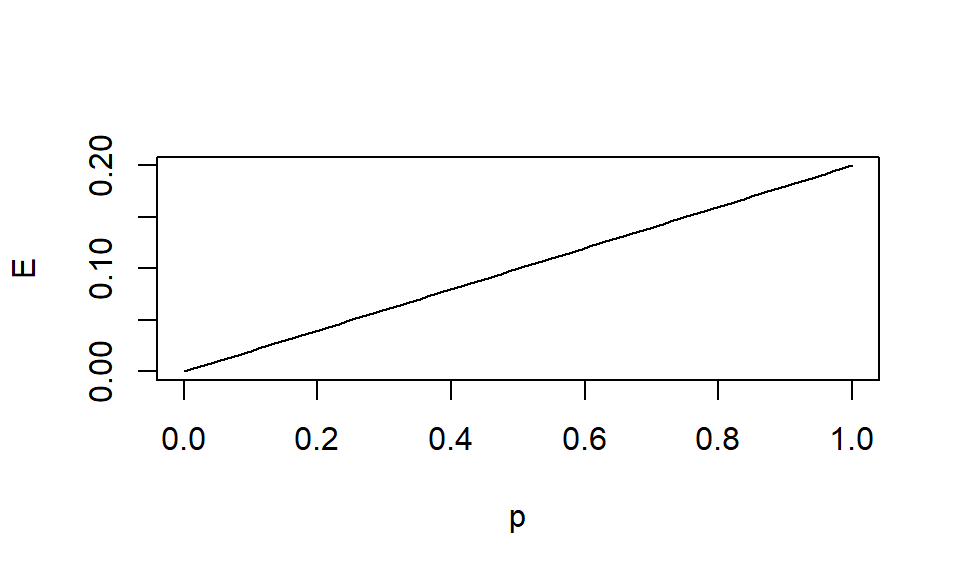
Plot the relationship b/w \(p\) and \(ep\)
E <- e*p
plot(E ~ p, type = "l")
R exercise: extinction
Draw how extinction rate changes over \(p\)
Plot the relationship b/w \(p\) and \(ep\)
E <- e*p
plot(E ~ p, type = "l")
R exercise: m & e
Draw how colonization & extinction rates change over \(p\)
plot(M ~ p, type = "l")
lines(E ~ p, col = "red")
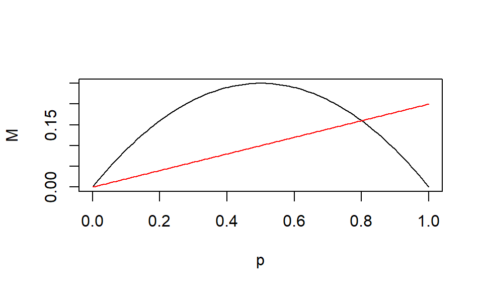
Equilibrium occupancy

- With \(p\) below the intersection, occupancy ___
- With \(p\) above the intersection, occupancy ___
Equilibrium occupancy
\[
\frac{dp}{dt} = mp(1-p) - ep
\]

Equilibrium occupancy
How to get equilibrium occupancy?
Equilibrium occupancy
Solve the following eq. about \(p\)
\[
\begin{align}
\frac{dp}{dt} &= cp(1-p) - ep = 0\\
p^* &= ...\\
\end{align}
\]
Equilibrium occupancy
Solve the following eq. about \(p\)
\[
p^* = 1 - \frac{e}{m}
\]
Condition for persistence
For a metapopulation to persist, \(p^*\) > 0
\[
p^* = 1 - \frac{e}{m} > 0
\]
Condition for persistence
For a metapopulation to persist, \(p^*\) must exceed zero, meaning
\[
m > e
\]
Colonization rate \(m\) must exceed extinction rate \(e\)
Link to logistic model
The Levins Metapopulation Model:
\[
\frac{dp}{dt} = mp(1-p) - ep
\]
can be transformed to:
\[
\frac{dp}{dt} = (m-e)p(1-\frac{p}{1-\frac{e}{m}})
\]
Link to logistic model
Express differently
\[
\frac{dp}{dt} = (m-e)p(1-\frac{p}{1-\frac{e}{m}})
\]
Let (1) \(p = N\), (2) \(m-e = r\), and (3) \(1-\frac{e}{m} = K\)
\[
\frac{dN}{dt} = rN(1-\frac{N}{K})
\]
Thus, the Levins metapopulation model can be seen as a logistic model at a different spatial scale
NOTE: not identical as \(0 \le p \le 1\)
Assumptions
Classical metapopulation assumes
- No variation in population size
- Immigration from within-metapopulation sources
- Random colonization & extinction
- Dispersal do NOT affect population dynamics
Mainland-island metapopulation
Mainland-island metapopulation model
One of the assumptions in the Levins metapopulation model is equal population size
The mainland-island metapopulation model is on the other extreme
Levins vs. mainland-island
Assumptions
- One LARGE population (the mainland) that never goes extinct
- Immigration from the mainland to islands only
- Random extinctions on islands
R exercise: colonization
Draw how colonization/extinction rate changes over \(p\)
Create \(p\), \(m\) and \(e\)
p <- seq(from = 0, to = 1, length = 100)
m <- e <- 1
R exercise: colonization
Draw how colonization/extinction rate changes over \(p\)
Create \(m(1-p)\) and \(ep\)
R exercise: colonization
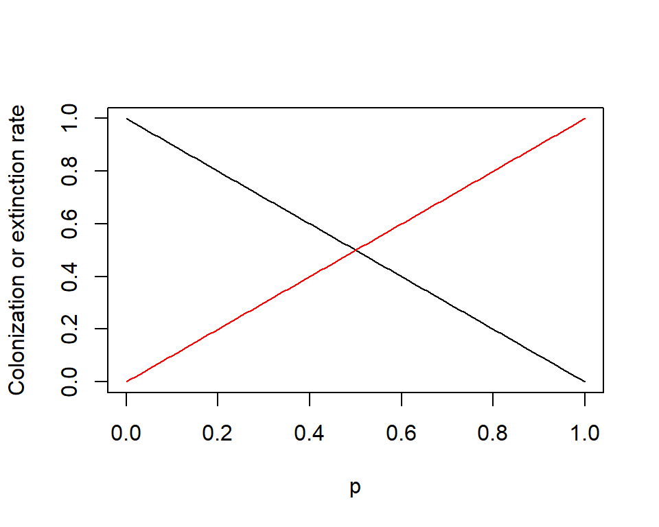
Plot \(m(1-p)\) and \(ep\)
plot(M ~ p, type = "l", ylab = "Colonization or extinction rate")
lines(E ~ p, col = "red")
Equilibrium
The mainland-island metapopulation model:
\[
\frac{dp}{dt} = m(1-p) - ep
\]
The equilibrium occupancy \(p^*\) is
\[
p^* = ...
\]
Equilibrium
\[
p^* = \frac{m}{m+e}
\]

Condition for persistence
For a metapopulation to persist, \(p^* > 0\)
\(\frac{m}{m+e} > 0\), i.e., \(m > 0\)
Condition for persistence
When \(m > 0\), there is a persistent supply of immigrants from the mainland
- the metapopulation never goes extinct
- higher extinction rate \(e\) cannot lead to the metapopulation extinction
More complexity
The metapopulation models are clearly oversimplified
In particular…
- Random extinction
- Random colonization
Assumptions
Random extinction
Population size varies in nature and influences local extinction risk
Random colonization
Organisms have limited dispersal capability
Proxies
Focus on a single habitat patch and think colonization into and extinction of the patch

Proxies
Habitat size
Extinction probability decreases with increasing habitat size

Rationale: habitat size
In a large habitat…
- population size is larger
- more refuge
Proxies
Isolation
Colonization probability decreases with increasing isolation
Rationale: isolation
In a isolated habitat,
- dispersal is more costly & risky
- dispersing individuals are less likely to arrive
Measures of isolation
- distance to the nearest neighbor
- distance weighted measure
Empirical approach
When studying real organisms…
- survey presence/absence of the species \(y_i\) at each habitat
- relate to habitat size and isolation (and other factors)
\[
y_i = f(habitat~size, isolation)
\]
Reality
More reality might be needed for empirical studies
- matrix permeability
- wind
- current
- species interactions
Gap
Theory: metapopulation-level occupancy
Empirical: patch-level occupancy