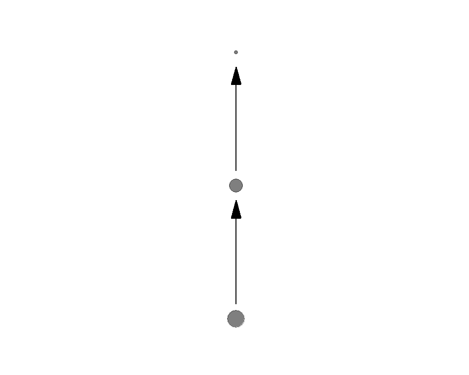
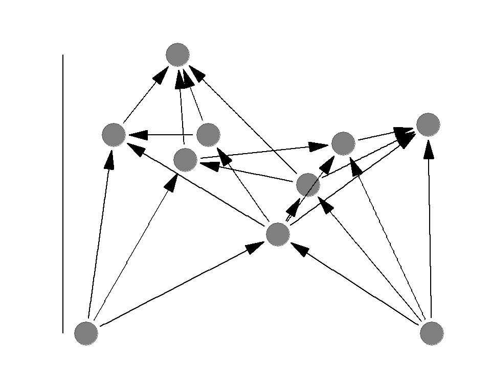
Trophic position
Trophic position (TP) is the vertical position in a food web
- Basal species have a value of one (e.g., plants)
- Primary consumers have a value of two (e.g., hevivores)

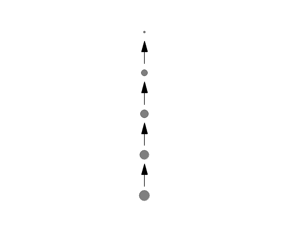
Trophic position
Trophic position (TP) is the vertical position in a food web
- Predators have continuous values (1 < TP)
- How would you define them?
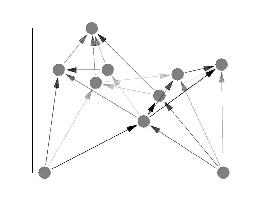
Fractional trophic position
\[
TP_i = 1 + \sum_{i}^{S}{F_{j}TP_{j}}
\] Consumer
- \(TP_{i}\) Trophic position of species \(i\)
Prey
- \(F_{j}\) Fraction of species j in the diet
- \(TP_{j}\) Trophic position of species j
Pauly and Palomales 2005, Bulletin of Marine Science
Fractional trophic position
\[
TP_i = 1 + \sum_{i}^{S}{F_{j}TP_{j}}
\]

Food chain length
Food chian length is the TP of the apex predator

Why food chain length is important
Food chain length is a summary measure of a food web
Why is it important?
Why food chain length is important
Food chain length influences
- Energy flows\(^1\)
- Top down control\(^2\)
- Primary production\(^2\)
- Atomospheric carbon exchange\(^2\)
- Contaminant concentrations in top predators\(^3\)
\(^1\)Wang et al. 2018 Ecology Letters \(^2\)Pace et al. 1998 TREE \(^3\)Kidd et al. 1998 CFJAS
Measuring food chain length
Methods
There are many methods, but stable isotopes (nitrogen) is the most common approach
Method 1
Connectance web
- Binary interactions (0 or 1)
- Ignores energy flow

Method 2
Energy web
- Quantitative interactions
- Extremely time consuming
Method 3
Stable isotopes
- Composite measure of food chain length
- (Relatively) easy to measure
- Food web structure itself is unknown
Food chain length with stable isotopes
Collect stable isotope data (nitrogen) for the baseline and top predator
Baseline can be producer or primary consumer
Equation
Food chain length (top predator’s TP) is calculated as:
\[
FCL = \frac{\delta ^{15}N_{predator} - \delta ^{15}N_{base}}{\Delta_N} + TP_{base}
\]
\(\Delta_N\) is TEF for nitrogen, and \(TP_{base}\) is the trophic position of the base species (1.0 or 2.0)
The advantage
Recall: stable isotopes are the mixed signature of prey resources
It can account for complicated food web structure without knowing the specifics
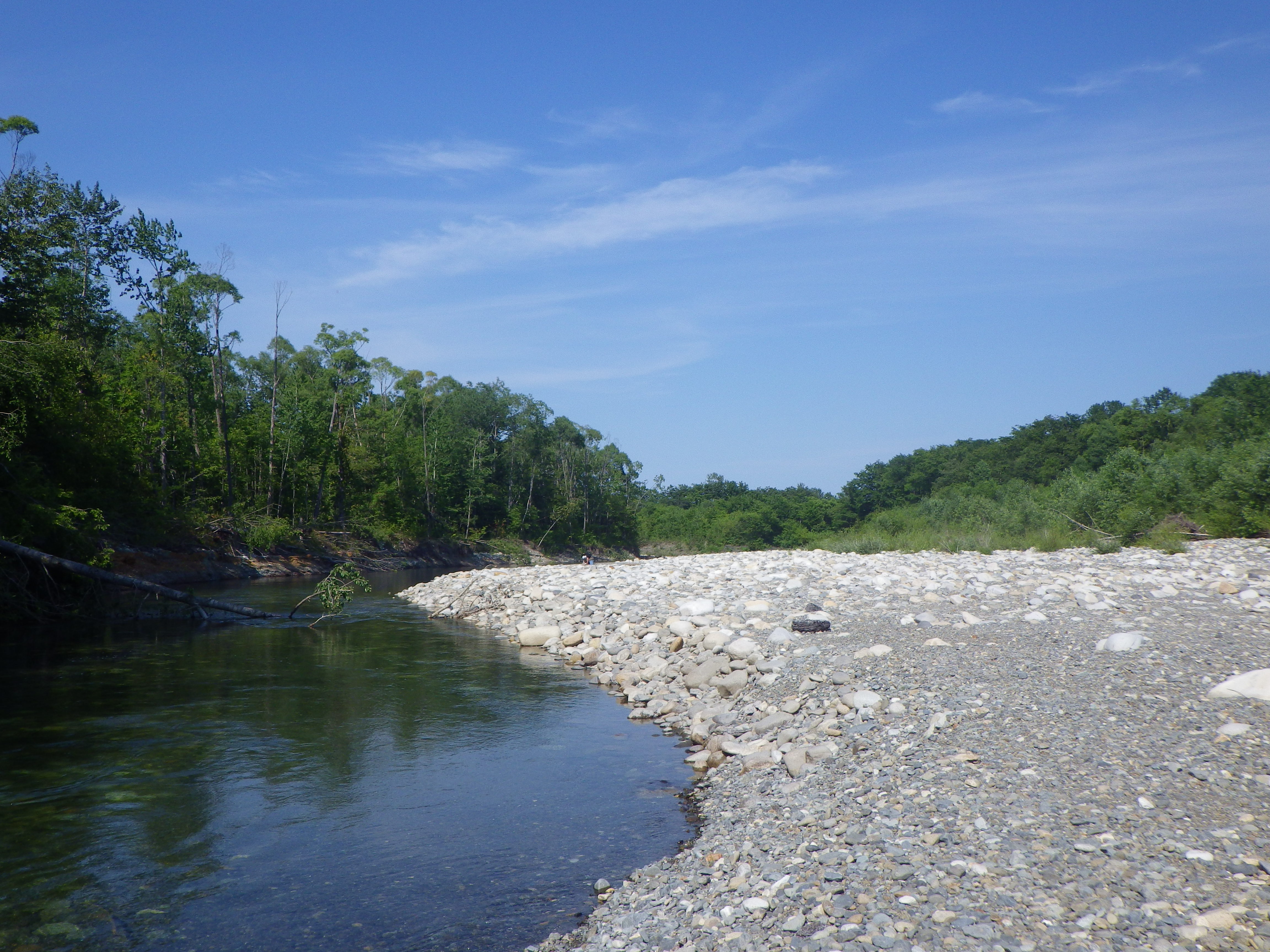
Tottabetsu river
Tottabetsu River, Japan
Ground beetles
Ground beetle - generalist predator
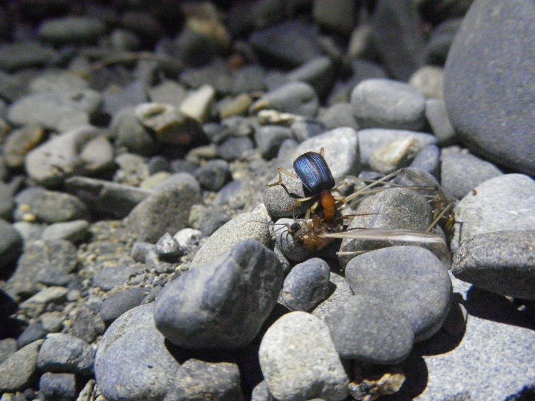 Brachinus stenoderus
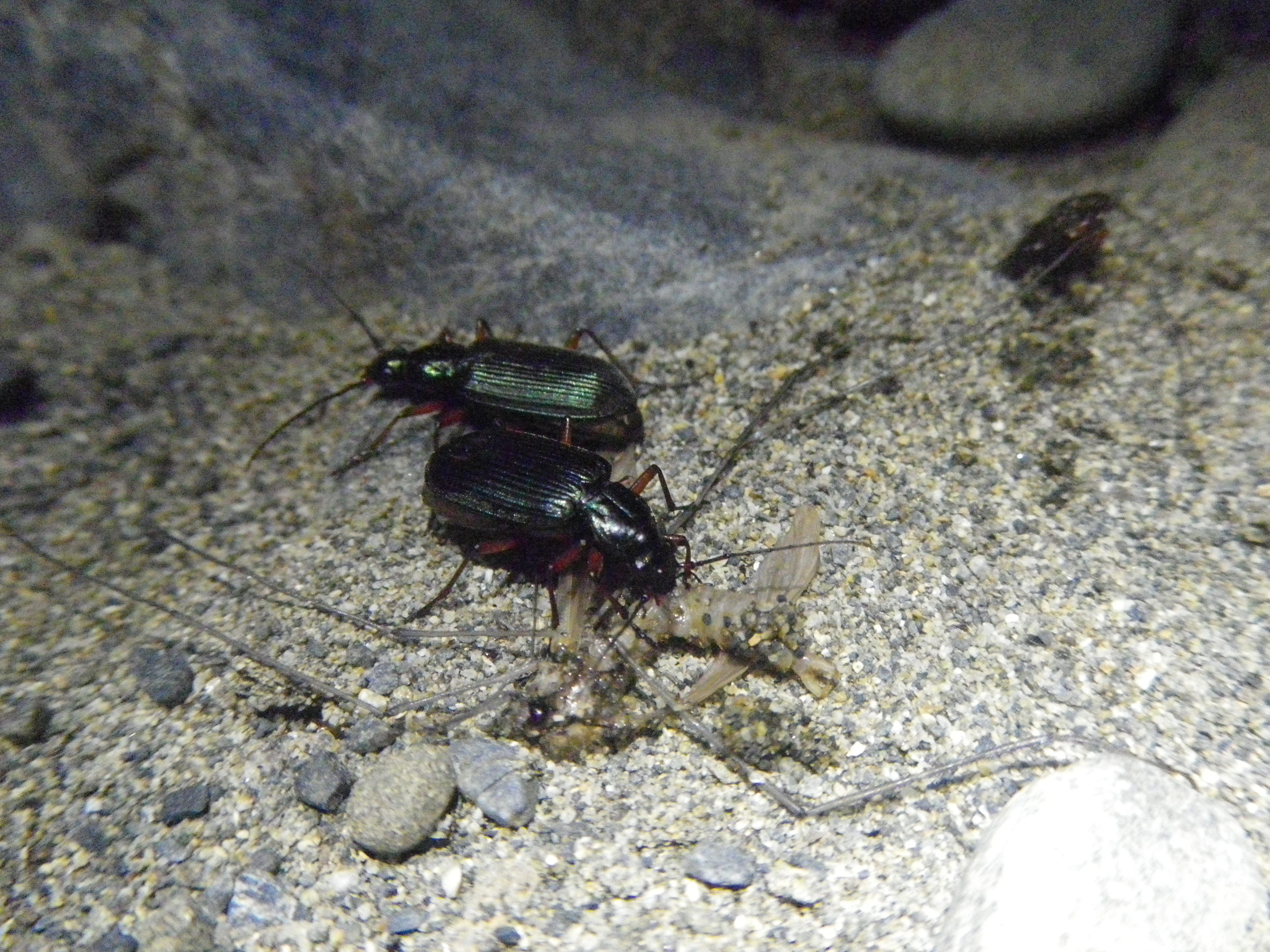 Lithochlaenius noguchii
R exercise: data
Download sample_data.csv and read it into R
dat <- read.csv("data/sample_data.csv")
head(dat)
##         site     date     species   d13C  d15N
## 1 tottabetsu 6/9/2014 grasshopper -28.03 -0.04
## 2 tottabetsu 6/9/2014 grasshopper -27.86  2.53
## 3 tottabetsu 6/9/2014 grasshopper -28.18  0.99
## 4 tottabetsu 6/9/2014 grasshopper -28.24  0.81
## 5 tottabetsu 8/9/2014 grasshopper -26.94  0.23
## 6 tottabetsu 8/9/2014 grasshopper -27.92  1.65
R exercise: mean N
Calculate mean \(\delta ^{15}N\) for each taxon
library(tidyverse)

datN = dat %>%
  group_by(species) %>% # grouping by 'species'
  summarize(meanN = mean(d15N)) # calculate means for each group

datN
## # A tibble: 3 x 2
##   species      meanN
##   <chr>        <dbl>
## 1 B_stenoderus 5.88
## 2 grasshopper  0.933
## 3 L_noguchii   5.06
R exercise: trophic position
\[
TP_{predator} = \frac{\delta ^{15}N_{predator} - \delta ^{15}N_{base}}{\Delta_N} + TP_{base}
\]
Calculate trophic positions of L. noguchii and B.stenoderus
*\(\Delta_{N} = 3.4\) and \(TP_{base} = 2\) for this example
Ngh <- datN$meanN[which(datN$species == "grasshopper")]
Nln <- datN$meanN[which(datN$species == "L_noguchii")]
Nbs <- datN$meanN[which(datN$species == "B_stenoderus")]

fcl <- function(Nbase, Ntop, deltaN, TPbase) {
  y <- (Ntop - Nbase)/deltaN + TPbase
  return(y)
}

TPln <- fcl(Nbase = Ngh, Ntop = Nln, deltaN = 3.4, TPbase = 2)
TPbs <- fcl(Nbase = Ngh, Ntop = Nbs, deltaN = 3.4, TPbase = 2)
R exercise: trophic position
Check values
L. noguchii: TP = 3.21
B. stenoderus: TP = 3.46
## [1] 3.213063
## [1] 3.456478
Long lasting debate
Food chain length varies in nature
What determines food chain length?
Basal resource availability
The productivity hypothesis predicts that food chain length should increase with increasing resource availability - why?
Rationale
Energy would be lost through predation
Post (2002) summarized energetic efficiency in predator-prey interactions
- Average: 10%
- Range: 5 - 50%
Post 2002, TREE 6: 269-277
Diminishing energy
Energy available to the top predator will be limited by basal resource availability or energetic efficiency
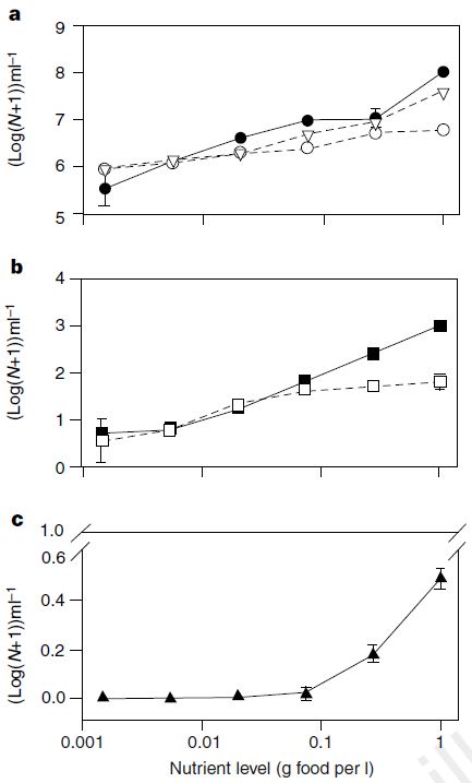
Empirical evidence
Highly controlled microbial system
As nutrient supply increased, population abundance of predatory ciliate increased
- Basal bacterium Serratia marcescens
- Bacterivorous ciliate Colpidium striatum
- Predatory ciliate Didinium nasutum
Kaunzinger and Morin 1998, Nature
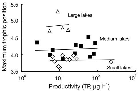
Counter evidence
Natural lakes
No response of food chain length to nutrient levels
- Top predators vary by lakes
- Greater diversity
Post et al. 2000, Nature
Theory impaired?
Contradicting results in experimental and natural systems
Why does the difference emerge?
Food web structure
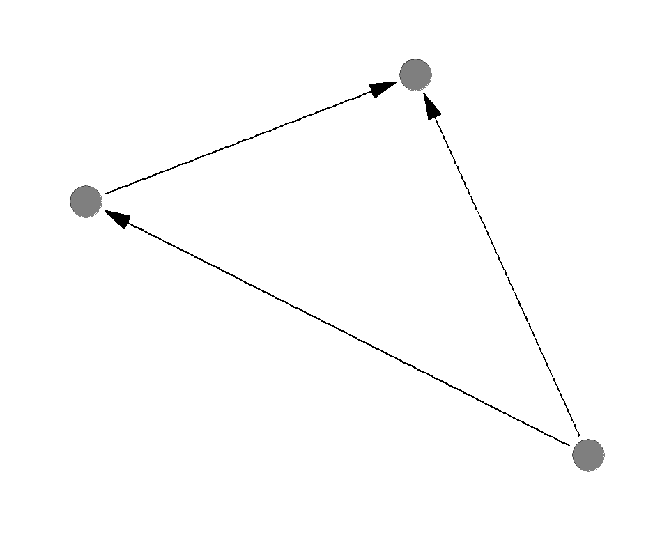
Intraguild predation
Predation on the species that shares a prey item(s)
Intraguild predation
Intraguild predation can drive intraguild prey extinction
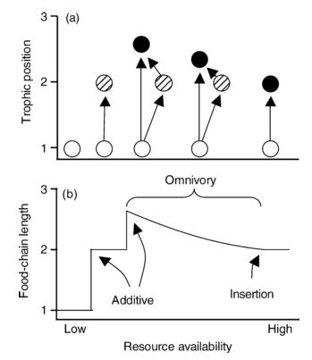
Resource availability
- Low: predator and/or consumer cannot invade into the system
- Medium: predator and consumer coexist
- High: predator extirpate consumer
Post & Takimoto. 2007, Oikos
Theoretical evidence
Ward et al. 2017, Nature Communications
The dynamic stability hypothesis
The dynamic stability hypothesis predicts that food chain length will decrease with increasing disturbance frequency/intensity - why?
Pimm and Lawton 1977, Nature
Rationale
Long food chains take time to recover - frequent/intense disturbance will inhibit recovery
Pimm and Lawton 1977, Nature
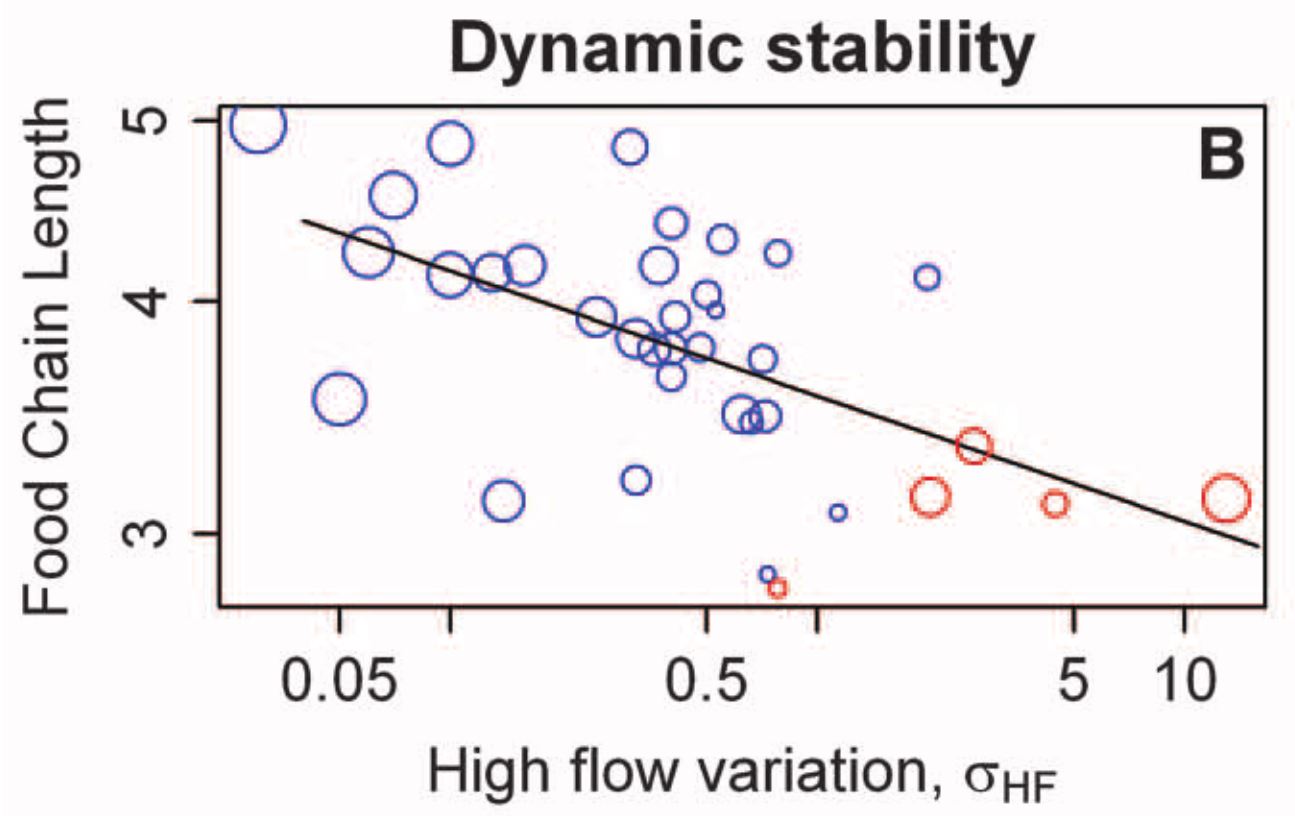
Empirical evidence
Often tested in rivers
US river ecosystem
- River flows stongly influences ecological communities
- Flow variation was quantified with long-term discharge records
Sabo et al. 2010, Science
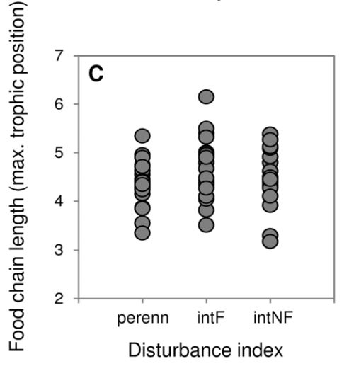
Counter evidence
Often tested in rivers
Australian river ecosystem
- River flows stongly influences ecological communities
- Flow regimes were categorized into three levels
Warfe et al. 2013, Plos One
Theory impaired?
Contradicting results in different regions
Why does the difference emerge?
Intraguild predation
Again, theory suggests intraguild predation may mediate the effect of disturbance
Disturbance
- Low: coexistence of IG-prey and IG-predator depends on the strength of IG predation
- Medium: IG-prey and IG-predator coexist
- High: no species can invade into the system
Takimoto et al. 2012, Ecological Research
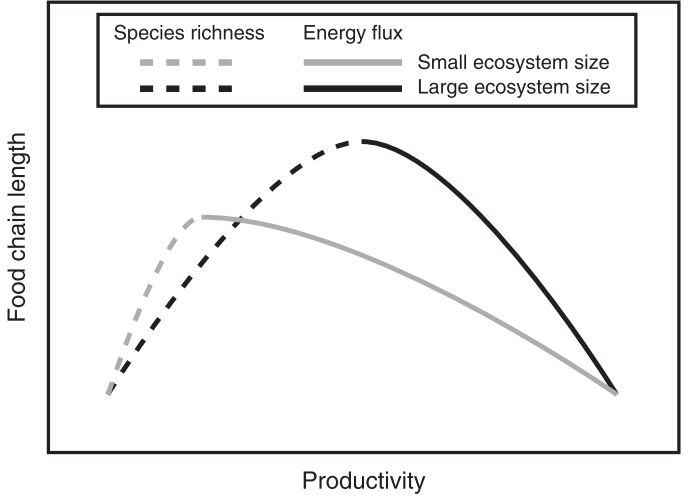
The ecosystem size hypothesis
The ecosystem size hypothesis predicts long food chains in large ecosystems (area or volume) - why?
Rationale
Multiple possibilities
- More space, more refugia
- Habitat heterogeneity
- More species
- and more…
i.e., mechanisms are unclear
Empirical evidence
Ample empirical evidence - lakes, ponds, and islands
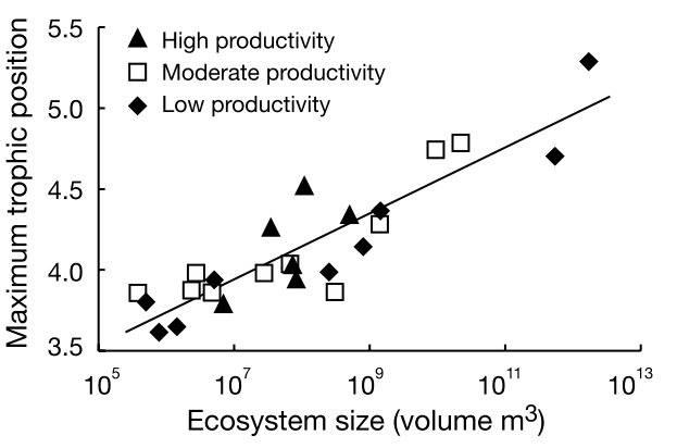
Post et al. 2000, Nature