5 Vector-Raster Interactions
5.1 Learning objectives
Understand the fundamentals of vector–raster interaction and analysis
Learn how to extract and append raster-derived attributes to vector data
Visualize the results of vector–raster analysis using effective mapping techniques
In this chapter, we will work with the following packages. Before starting any exercises, make sure to run the following code.
if (!require(pacman)) install.packages("pacman")

pacman::p_load(tidyverse,
               sf,
               terra,
               tidyterra,
               exactextractr)
5.2 Interations between vector and raster data
In ecological data analysis, it is common to relate ecological responses (e.g., species richness) to environmental variables. To do this effectively, we often need to extract values from raster layers at specific locations, such as survey sites (points) or areas (polygons). This step allows us to link ecological observations with spatial environmental data for further analysis. In this exercise, we will use fish survey sites and county polygons to extract environmental variables from raster data.
To get started, read the following datasets into R to perform the analysis:
5.3 Point-wise extraction
Let’s perform point-wise extraction of precipitation values at survey site locations.
To explore the spatial patterns and get a sense of the data, we will first visualize the raster precipitation data using tidyterra::geom_spatraster() and overlay the survey sites using ggplot2::geom_sf().
ggplot() +
  geom_spatraster(data = spr_prec_nc) +
  geom_sf(data = sf_site) +
  scale_fill_viridis_c() + # change color palette for raster
  theme_bw()
To extract raster values at the survey sites, we will use the terra::extract() function.
This function retrieves the values of one or more raster layers at the locations specified by spatial vector data, such as points or polygons.
In our case, it will return the precipitation value at each survey site location.
Since the output of terra::extract() with bind = TRUE is a class of SpatVector that includes geometry but is not yet an sf object, we convert it back to an sf object using sf::st_as_sf() (using %>%, these steps can be done in one step).
# # The following code works exactly as:
# spr_site_prec <- extract(x = spr_prec_nc,
#                          y = sf_site,
#                          bind = TRUE)
#
# sf_site_prec <- st_as_sf(spr_site_prec)

(sf_site_prec <- extract(x = spr_prec_nc,
                         y = sf_site,
                         bind = TRUE) %>%
   st_as_sf())
## Simple feature collection with 122 features and 2 fields
## Geometry type: POINT
## Dimension: XY
## Bounding box: xmin: -84.02452 ymin: 34.53497 xmax: -76.74611 ymax: 36.54083
## Geodetic CRS: WGS 84
## First 10 features:
## site_id precipitation geometry
## 1 finsync_nrs_nc-10013 1349.4 POINT (-81.51025 36.11188)
## 2 finsync_nrs_nc-10014 1121.5 POINT (-80.35989 35.87616)
## 3 finsync_nrs_nc-10020 1297.3 POINT (-81.74472 35.64379)
## 4 finsync_nrs_nc-10023 1162.0 POINT (-82.77898 35.6822)
## 5 finsync_nrs_nc-10024 1302.0 POINT (-77.75384 35.38553)
## 6 finsync_nrs_nc-10027 1741.5 POINT (-83.69678 35.02467)
## 7 finsync_nrs_nc-10029 1224.3 POINT (-80.65668 35.16119)
## 8 finsync_nrs_nc-10034 1813.2 POINT (-82.04497 36.09917)
## 9 finsync_nrs_nc-10041 1141.3 POINT (-80.46558 35.04365)
## 10 finsync_nrs_nc-10049 1444.7 POINT (-77.96322 34.58249)This allows for seamless spatial operations and visualization downstream. Since our point data now include precipitation values, we can represent the survey sites with colors that reflect the precipitation gradient.
ggplot() +
  geom_sf(data = sf_nc_county,       # Plot county boundaries as a grey background
          fill = "grey") +
  geom_sf(data = sf_site_prec,       # Plot survey points colored by precipitation
          aes(color = precipitation)) +
  scale_color_viridis_c() +          # Apply a perceptually uniform color scale
  theme_bw()                        # Use a clean black-and-white theme
5.4 Zonal statistics
Zonal statistics in GIS refers to the process of summarizing raster values within the boundaries of defined zones, typically represented by polygons. For example, you might calculate the average precipitation within each watershed or administrative boundary. This is commonly done by overlaying polygon features onto a raster layer and computing summary statistics (e.g., mean, sum, min, max) for all raster cells that fall within each polygon.
5.4.1 Polygon-based analysis
Traditional approach
The exactextractr package provides a suite of efficient and precise tools for performing zonal statistics, particularly when working with raster and polygon data.
In the following example, we will use exact_extract() to calculate the mean precipitation within each county polygon.
However, before performing zonal statistics, it is critical to ensure that both the raster and vector layers use a projected CRS – not a geographic one (like WGS 84 in degrees). This is because zonal statistics summarize values over areas, and accurate area-based calculations require linear units (e.g., meters), which are only meaningful in a projected CRS.
In this example, we first reproject the county polygon layer sf_nc_county into WGS 84 / UTM zone 17N (EPSG:32617), a projected CRS appropriate for central and eastern North Carolina.
Then, we use terra::project() to reproject the raster layer spr_prec_nc to match the polygon layer’s CRS.
The method = "bilinear" option is used for resampling continuous raster data (such as precipitation)3, providing smoother interpolation.
sf_nc_county_proj <- st_transform(sf_nc_county,
                                  crs = 32617)

spr_prec_nc_proj <- terra::project(x = spr_prec_nc,
                                   y = crs(sf_nc_county_proj),
                                   method = "bilinear")
With both layers now in a common projected CRS, we can proceed with zonal statistics, ensuring that area-weighted calculations are geometrically accurate.
In the code below, exact_extract() is used to calculate the mean precipitation within each county polygon (sf_nc_county_proj) from the reprojected raster spr_prec_nc_proj.
The argument fun = "mean" specifies that we want to compute the simple mean of all raster cell values that overlap each polygon.
The append_cols = TRUE option ensures that all original attributes from the sf_nc_county_proj object are retained in the output, which makes it easier to link the results back to the spatial features.
# NOTE: `progress = FALSE` turns off the progress bar for cleaner output
(df_prec_county <- exact_extract(x = spr_prec_nc_proj,
                                 y = sf_nc_county_proj,
                                 fun = "mean",
                                 append_cols = TRUE,
                                 progress = FALSE) %>%
   as_tibble() %>% # convert to tibble
   rename(precipitation = mean)) # rename the output column)
## # A tibble: 100 × 2
## county precipitation
## <chr> <dbl>
## 1 ashe 1366.
## 2 alleghany 1369.
## 3 surry 1217.
## 4 currituck 1281.
## 5 northampton 1179.
## 6 hertford 1239.
## 7 camden 1299.
## 8 gates 1275.
## 9 warren 1140.
## 10 stokes 1218.
## # ℹ 90 more rowsAlthough the output from exact_extract() is a regular data frame (not an sf object), we can easily merge the computed statistics back into the original spatial data using left_join()4.
This allows us to retain the spatial geometry of the county polygons while adding the precipitation values as new attributes.
In the example below, we assume that both the original sf object (sf_nc_county) and the extracted results (df_prec_county) share a common identifier column named county.
(sf_nc_county_prec <- sf_nc_county %>%
   left_join(df_prec_county,
             by = "county"))
## Simple feature collection with 100 features and 2 fields
## Geometry type: MULTIPOLYGON
## Dimension: XY
## Bounding box: xmin: -84.32377 ymin: 33.88212 xmax: -75.45662 ymax: 36.58973
## Geodetic CRS: WGS 84
## First 10 features:
## county precipitation geometry
## 1 ashe 1365.949 MULTIPOLYGON (((-81.47258 3...
## 2 alleghany 1368.901 MULTIPOLYGON (((-81.23971 3...
## 3 surry 1216.966 MULTIPOLYGON (((-80.45614 3...
## 4 currituck 1281.308 MULTIPOLYGON (((-76.00863 3...
## 5 northampton 1178.707 MULTIPOLYGON (((-77.21736 3...
## 6 hertford 1239.493 MULTIPOLYGON (((-76.74474 3...
## 7 camden 1299.447 MULTIPOLYGON (((-76.00863 3...
## 8 gates 1275.414 MULTIPOLYGON (((-76.56218 3...
## 9 warren 1139.996 MULTIPOLYGON (((-78.30849 3...
## 10 stokes 1217.916 MULTIPOLYGON (((-80.02545 3...The following plot uses ggplot2 to visualize the mean precipitation values calculated for each county.
The geom_sf() layer draws the county boundaries from the sf_nc_county_prec object, and the aes(color = precipitation) argument maps the precipitation values to a color gradient.
ggplot() +
  geom_sf(data = sf_nc_county_prec,
          aes(fill = precipitation)) +
  scale_fill_viridis_c() +
  theme_bw()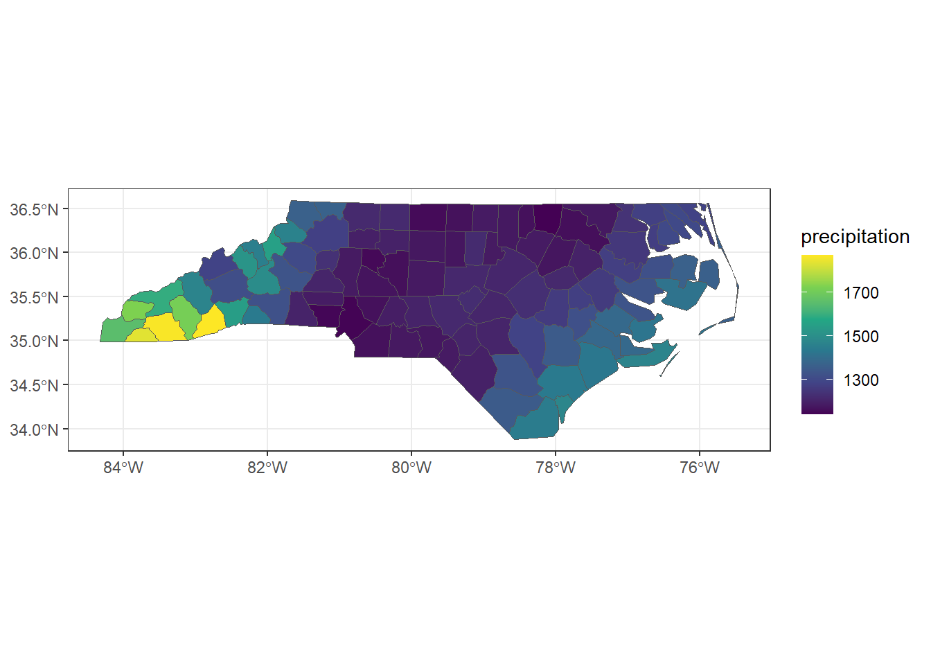
Alternative approach
The above example involved multiple steps to reproject both the raster and polygon layers into a common projected CRS, which is necessary for accurate area-based calculations.
However, the exact_extract() function provides a convenient alternative that avoids the need for explicit reprojection.
By specifying fun = "weighted_mean" and weights = "area", we instruct the function to calculate the mean precipitation for each polygon by weighting each raster cell’s contribution according to the fraction of its area that overlaps the polygon.
This internal weighting allows exact_extract() to produce geometrically accurate results even when the layers remain in a geographic CRS (e.g., WGS 84), which is especially useful when working with global datasets or when reprojection is impractical.
(df_prec_county_alt <- exact_extract(x = spr_prec_nc,
                                     y = sf_nc_county,
                                     fun = "weighted_mean",
                                     weights = "area",
                                     append_cols = TRUE,
                                     progress = FALSE) %>%
   as_tibble() %>% # convert to tibble
   rename(precipitation = weighted_mean)) # rename the output column
## # A tibble: 100 × 2
## county precipitation
## <chr> <dbl>
## 1 ashe 1366.
## 2 alleghany 1369.
## 3 surry 1217.
## 4 currituck 1281.
## 5 northampton 1179.
## 6 hertford 1239.
## 7 camden 1299.
## 8 gates 1275.
## 9 warren 1140.
## 10 stokes 1218.
## # ℹ 90 more rowsThe numbers produced by the area-weighted approach without reprojection may differ slightly from those obtained using fully projected layers.
In most cases, this difference is negligible, making the approximation both practical and efficient; especially when working across large spatial extents that span multiple UTM zones or even continents, where choosing a single appropriate projection becomes difficult.
In such cases, the ability of exact_extract() to apply area-based weights directly in geographic CRS is a major advantage, as it simplifies preprocessing and avoids potential distortions from inappropriate projections.
That said, if your analysis requires high spatial accuracy, for example, when modeling fine-scale ecological processes or when exact area measurements are critical, it is still recommended to reproject both raster and vector data to an appropriate projected CRS. Ultimately, the decision depends on the scale, purpose, and precision required by your specific application.
5.4.2 Buffer-based analysis
When linking environmental conditions to ecological data collected at survey sites, point-wise extraction is a straightforward and intuitive approach. However, environmental influences often operate at broader spatial scales. In such cases, buffer-based extraction may be more appropriate.
Like other zonal statistics, buffer analysis assumes a planar coordinate system, so it is important to first transform the data to a projected CRS.
Once projected, you can generate buffers around the survey sites using the sf::st_buffer() function.
sf_site_proj <- sf_site %>%
  st_transform(crs = 32617)

sf_site_buff_proj <- sf_site_proj %>%
  st_buffer(dist = 10000) # unit is meter in a projected CRS
The object sf_site_buff_proj is currently in a projected CRS (WGS 84 / UTM zone 17N; EPSG:32617), which is appropriate for spatial operations like buffering.
However, for visualization, a geodetic CRS such as WGS84 (EPSG:4326) is typically preferred.
Transform the object back to a geodetic CRS to ensure correct alignment with standard basemaps and mapping applications.
sf_site_buff <- sf_site_buff_proj %>%
  st_transform(crs = 4326)
Visualization allows you to see how buffers are created around the survey sites, helping to confirm that the spatial scale and geometry are appropriate for your analysis.
ggplot() +
  geom_sf(data = sf_nc_county,
          fill = "grey") +
  geom_sf(data = sf_site_buff,
          fill = "salmon") +
  geom_sf(data = sf_site) +
  theme_bw()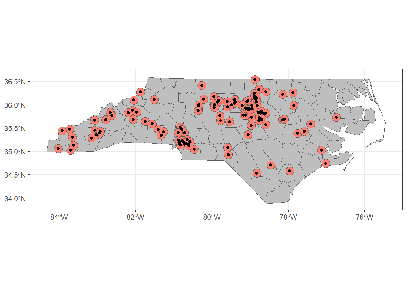
Taking zonal statistics is the same—after buffering in projected space, you can use the exactextractr::exact_extract() function to perform area-weighted extraction of raster values within each buffer zone.
df_prec_buff <- exact_extract(x = spr_prec_nc_proj,
                              y = sf_site_buff_proj,
                              fun = "mean",
                              append_cols = TRUE,
                              progress = FALSE) %>%
  as_tibble() %>%
  rename(precipitation = mean)
Like we did in the above examples, we can tie these extracted values back to the original point data by joining the summary statistics to the corresponding survey sites.
(sf_site_prec_buff <- sf_site %>%
   left_join(df_prec_buff,
             by = "site_id"))
## Simple feature collection with 122 features and 2 fields
## Geometry type: POINT
## Dimension: XY
## Bounding box: xmin: -84.02452 ymin: 34.53497 xmax: -76.74611 ymax: 36.54083
## Geodetic CRS: WGS 84
## # A tibble: 122 × 3
## site_id geometry precipitation
## <chr> <POINT [°]> <dbl>
## 1 finsync_nrs_nc-10013 (-81.51025 36.11188) 1419.
## 2 finsync_nrs_nc-10014 (-80.35989 35.87616) 1139.
## 3 finsync_nrs_nc-10020 (-81.74472 35.64379) 1313.
## 4 finsync_nrs_nc-10023 (-82.77898 35.6822) 1279.
## 5 finsync_nrs_nc-10024 (-77.75384 35.38553) 1296.
## 6 finsync_nrs_nc-10027 (-83.69678 35.02467) 1799.
## 7 finsync_nrs_nc-10029 (-80.65668 35.16119) 1203.
## 8 finsync_nrs_nc-10034 (-82.04497 36.09917) 1648.
## 9 finsync_nrs_nc-10041 (-80.46558 35.04365) 1160.
## 10 finsync_nrs_nc-10049 (-77.96322 34.58249) 1444.
## # ℹ 112 more rowsVisualize:
ggplot() +
  geom_sf(data = sf_nc_county,
          fill = "grey") +
  geom_sf(data = sf_site_prec_buff,
          aes(color = precipitation)) +
  scale_color_viridis_c() +
  theme_bw()
Fantastic!