6 Species Distribution Modeling
6.1 Learning objectives
Prepare ecological datasets for species-environment analyses
Integrate GIS-derived environmental variables with species occurrence data
Visualize and analyze relationships between environmental conditions and species distributions
In this chapter, we will work with the following packages. Before starting any exercises, make sure to run the following code.
if (!require(pacman)) install.packages("pacman")

pacman::p_load(tidyverse,
               ggeffects,
               sf,
               terra,
               tidyterra,
               exactextractr,
               mapview)
6.2 Linking GIS to ecology
So far, we have covered the fundamentals of GIS, but made only limited connections to ecological data. Now that we’ve developed core GIS skills, we are ready to link GIS-derived environmental variables to ecological patterns, such as species occurrence and distribution. Here, we’ll dip our toes into Species Distribution Modeling (SDM), a foundational approach in ecological modeling for understanding the relationships between species occurrences and the environment across broad spatial scales.
For this exercise, let’s use the fish data from finsyncR:
(df_finsync <- read_csv("data/data_finsync_nc.csv"))## # A tibble: 1,426 × 6
## site_id year date lon lat latin
## <chr> <dbl> <date> <dbl> <dbl> <chr>
## 1 finsync_nrs_nc-10013 2009 2009-06-27 -81.5 36.1 Clinostomus funduloides
## 2 finsync_nrs_nc-10013 2009 2009-06-27 -81.5 36.1 Etheostoma flabellare
## 3 finsync_nrs_nc-10013 2009 2009-06-27 -81.5 36.1 Hybopsis hypsinotus
## 4 finsync_nrs_nc-10013 2009 2009-06-27 -81.5 36.1 Lepomis auritus
## 5 finsync_nrs_nc-10013 2009 2009-06-27 -81.5 36.1 Moxostoma rupiscartes
## 6 finsync_nrs_nc-10013 2009 2009-06-27 -81.5 36.1 Nocomis leptocephalus
## 7 finsync_nrs_nc-10013 2009 2009-06-27 -81.5 36.1 Notropis chiliticus
## 8 finsync_nrs_nc-10013 2009 2009-06-27 -81.5 36.1 Semotilus atromaculatus
## 9 finsync_nrs_nc-10014 2009 2009-06-03 -80.4 35.9 Clinostomus funduloides
## 10 finsync_nrs_nc-10014 2009 2009-06-03 -80.4 35.9 Fundulus rathbuni
## # ℹ 1,416 more rowsAs outlined in Chapter 2, this dataset contains records of fish species observed at survey sites across North Carolina.
To better understand the structure of the data, let’s examine the first survey site (site_id == "finsync_nrs_nc-10013"):
(df_st1 <- df_finsync %>%
  filter(site_id == "finsync_nrs_nc-10013"))
## # A tibble: 8 × 6
## site_id year date lon lat latin
## <chr> <dbl> <date> <dbl> <dbl> <chr>
## 1 finsync_nrs_nc-10013 2009 2009-06-27 -81.5 36.1 Clinostomus funduloides
## 2 finsync_nrs_nc-10013 2009 2009-06-27 -81.5 36.1 Etheostoma flabellare
## 3 finsync_nrs_nc-10013 2009 2009-06-27 -81.5 36.1 Hybopsis hypsinotus
## 4 finsync_nrs_nc-10013 2009 2009-06-27 -81.5 36.1 Lepomis auritus
## 5 finsync_nrs_nc-10013 2009 2009-06-27 -81.5 36.1 Moxostoma rupiscartes
## 6 finsync_nrs_nc-10013 2009 2009-06-27 -81.5 36.1 Nocomis leptocephalus
## 7 finsync_nrs_nc-10013 2009 2009-06-27 -81.5 36.1 Notropis chiliticus
## 8 finsync_nrs_nc-10013 2009 2009-06-27 -81.5 36.1 Semotilus atromaculatusThe dataset follows the “tidy” data format, where each column contains a single type of information and each row represents a single observation (see here for more details). While this format is recommended for the initial data entry, it sometimes inconvenient for data analysis - in what follows, let me walk you through how we convert it to an analysis-ready format.
6.2.1 Preparing ecological data
As an example, let’s model the distribution of a single species from our dataset as a function of air temperature—specifically, how the probability of occurrence changes along a temperature gradient. This is the question we aim to address through SDM, and the following exercise is designed to achieve this aim.
The first step is data wrangling. Ecological datasets are often not in an analysis-ready format, and ours is no exception. In this dataset, we know which species were present at each survey site, but absence is not explicitly recorded; species simply do not appear in the data for sites where they were not observed.
To model a species’ response to environmental conditions, we need to compare sites where the species was observed to those where it was absent. This contrast enables us to estimate how environmental variables—like air temperature—influence the probability of species occurrence. Therefore, we must reshape the dataset to include complete presence/absence information for a single species across all survey sites.
The goal is to create a dataframe listing species presence/absence across all survey sites.
To make it clear that each row represents a presence record, let me add a column of “presence” – then we’ll use the function dplyr::pivot_wider() to complete this task:
df_finsync %>%
  mutate(presence = 1) %>% # all recorded species are "presence" = 1
  pivot_wider(id_cols = c(site_id, lon, lat),
              names_from = latin,
              values_from = presence)
## # A tibble: 122 × 133
## site_id lon lat Clinostomus funduloi…¹ Etheostoma flabellar…²
## <chr> <dbl> <dbl> <dbl> <dbl>
## 1 finsync_nrs_nc-100… -81.5 36.1 1 1
## 2 finsync_nrs_nc-100… -80.4 35.9 1 NA
## 3 finsync_nrs_nc-100… -81.7 35.6 1 1
## 4 finsync_nrs_nc-100… -82.8 35.7 NA 1
## 5 finsync_nrs_nc-100… -77.8 35.4 NA NA
## 6 finsync_nrs_nc-100… -83.7 35.0 NA NA
## 7 finsync_nrs_nc-100… -80.7 35.2 1 NA
## 8 finsync_nrs_nc-100… -82.0 36.1 NA NA
## 9 finsync_nrs_nc-100… -80.5 35.0 NA 1
## 10 finsync_nrs_nc-100… -78.0 34.6 NA NA
## # ℹ 112 more rows
## # ℹ abbreviated names: ¹`Clinostomus funduloides`, ²`Etheostoma flabellare`
## # ℹ 128 more variables: `Hybopsis hypsinotus` <dbl>, `Lepomis auritus` <dbl>,
## # `Moxostoma rupiscartes` <dbl>, `Nocomis leptocephalus` <dbl>,
## # `Notropis chiliticus` <dbl>, `Semotilus atromaculatus` <dbl>,
## # `Fundulus rathbuni` <dbl>, `Ambloplites rupestris` <dbl>,
## # `Campostoma anomalum` <dbl>, `Catostomus commersonii` <dbl>, …In this case, we set id_cols = c(site_id, lon, lat), names_from = latin, and values_from = presence.
By setting these arguments, the function will return a dataframe where each row represents a survey site (a unique combination of site_id, lon, and lat), each column corresponds to a unique species, and the cell values indicate whether each species was present (1) or absent (NA) at that site.
When species are not recorded at a given site, the function returns NA because there is no such combination of species and site in the original data – however, for the purpose of statistical modeling, we want to treat these as zeros (= absence).
An additional argument, values_fill = 0, will achieve this by filling all NA values in the output dataframe with 0, allowing us to interpret the data as complete presence/absence records across all sites and species.
df_finsync %>%
  mutate(presence = 1) %>% # all recorded species are "presence" = 1
  pivot_wider(id_cols = c(site_id, lon, lat),
              names_from = latin,
              values_from = presence,
              values_fill = 0)
## # A tibble: 122 × 133
## site_id lon lat Clinostomus funduloi…¹ Etheostoma flabellar…²
## <chr> <dbl> <dbl> <dbl> <dbl>
## 1 finsync_nrs_nc-100… -81.5 36.1 1 1
## 2 finsync_nrs_nc-100… -80.4 35.9 1 0
## 3 finsync_nrs_nc-100… -81.7 35.6 1 1
## 4 finsync_nrs_nc-100… -82.8 35.7 0 1
## 5 finsync_nrs_nc-100… -77.8 35.4 0 0
## 6 finsync_nrs_nc-100… -83.7 35.0 0 0
## 7 finsync_nrs_nc-100… -80.7 35.2 1 0
## 8 finsync_nrs_nc-100… -82.0 36.1 0 0
## 9 finsync_nrs_nc-100… -80.5 35.0 0 1
## 10 finsync_nrs_nc-100… -78.0 34.6 0 0
## # ℹ 112 more rows
## # ℹ abbreviated names: ¹`Clinostomus funduloides`, ²`Etheostoma flabellare`
## # ℹ 128 more variables: `Hybopsis hypsinotus` <dbl>, `Lepomis auritus` <dbl>,
## # `Moxostoma rupiscartes` <dbl>, `Nocomis leptocephalus` <dbl>,
## # `Notropis chiliticus` <dbl>, `Semotilus atromaculatus` <dbl>,
## # `Fundulus rathbuni` <dbl>, `Ambloplites rupestris` <dbl>,
## # `Campostoma anomalum` <dbl>, `Catostomus commersonii` <dbl>, …Lastly, let’s focus on a single species for this exercise.
We’ll extract the presence/absence information for Redbreast Sunfish (Lepomis auritus) along with the corresponding site_id and longitude (lon) / latitude (lat).
This subset will serve as the response variable in our upcoming analysis, allowing us to examine how environmental conditions shape the distribution of this focal species across the survey sites.
## assign df_rbs
(df_rbs <- df_finsync %>%
  mutate(presence = 1) %>% # all recorded species are "presence" = 1
  pivot_wider(id_cols = c(site_id, lon, lat),
              names_from = latin,
              values_from = presence,
              values_fill = 0) %>%
  select(site_id,
         lon,
         lat,
         "Lepomis auritus") %>%
  rename(y = "Lepomis auritus")) # rename column "Lepomis auritus" to y
## # A tibble: 122 × 4
## site_id lon lat y
## <chr> <dbl> <dbl> <dbl>
## 1 finsync_nrs_nc-10013 -81.5 36.1 1
## 2 finsync_nrs_nc-10014 -80.4 35.9 0
## 3 finsync_nrs_nc-10020 -81.7 35.6 0
## 4 finsync_nrs_nc-10023 -82.8 35.7 1
## 5 finsync_nrs_nc-10024 -77.8 35.4 0
## 6 finsync_nrs_nc-10027 -83.7 35.0 0
## 7 finsync_nrs_nc-10029 -80.7 35.2 0
## 8 finsync_nrs_nc-10034 -82.0 36.1 0
## 9 finsync_nrs_nc-10041 -80.5 35.0 1
## 10 finsync_nrs_nc-10049 -78.0 34.6 0
## # ℹ 112 more rows6.2.2 Linking to the environment
To see the influence of air temperature on fish distribution (assuming that it influences fish via changes in water temperature), we need to tie the occurrence dataframe df_rbs to air temperature at each survey site.
To perform this, we’ll use the point-wise extraction method introduced in Chapter 5.
This method requires an sf object containing the spatial coordinates of each survey site, because spatial extraction (e.g., using terra::extract()) operates on geometries.
So first, we’ll create an sf object listing unique site coordinates along with site_id.
Here’s a code example that outlines this step:
sf_rbs <- df_rbs %>%
  st_as_sf(coords = c("lon", "lat"),
           crs = 4326)
Point-wise extraction can be done with the procedure outlined in Section 5.3 in Chapter 5. This allows us to extract raster values—such as air temperature—at the locations of our survey sites.
To begin, we’ll read the raster layer that contains air temperature data, then use the terra::extract() function to obtain values at each survey site using the sf object we created earlier.
## read temperature raster
spr_tmp_nc <- rast("data/spr_tmp_nc.tif")

## extract values at the survey sites
(sf_rbs_tmp <- extract(x = spr_tmp_nc,
                       y = sf_rbs,
                       bind = TRUE) %>%
   st_as_sf())
## Simple feature collection with 122 features and 3 fields
## Geometry type: POINT
## Dimension: XY
## Bounding box: xmin: -84.02452 ymin: 34.53497 xmax: -76.74611 ymax: 36.54083
## Geodetic CRS: WGS 84
## First 10 features:
## site_id y temperature geometry
## 1 finsync_nrs_nc-10013 1 13.65 POINT (-81.51025 36.11188)
## 2 finsync_nrs_nc-10014 0 15.15 POINT (-80.35989 35.87616)
## 3 finsync_nrs_nc-10020 0 14.25 POINT (-81.74472 35.64379)
## 4 finsync_nrs_nc-10023 1 12.65 POINT (-82.77898 35.6822)
## 5 finsync_nrs_nc-10024 0 16.45 POINT (-77.75384 35.38553)
## 6 finsync_nrs_nc-10027 0 13.45 POINT (-83.69678 35.02467)
## 7 finsync_nrs_nc-10029 0 15.85 POINT (-80.65668 35.16119)
## 8 finsync_nrs_nc-10034 0 9.35 POINT (-82.04497 36.09917)
## 9 finsync_nrs_nc-10041 1 16.15 POINT (-80.46558 35.04365)
## 10 finsync_nrs_nc-10049 0 16.85 POINT (-77.96322 34.58249)For analysis, it’s convenient to have the data in tibble format, especially since the geometry column from the sf object is not needed for statistical modeling.
We can easily convert the spatial object to a regular tibble using tidyr::as_tibble(), which drops the geospatial infromation by default (e.g., CRS).
(df_rbs_tmp <- as_tibble(sf_rbs_tmp) %>%
  select(-geometry))
## # A tibble: 122 × 3
## site_id y temperature
## <chr> <dbl> <dbl>
## 1 finsync_nrs_nc-10013 1 13.6
## 2 finsync_nrs_nc-10014 0 15.1
## 3 finsync_nrs_nc-10020 0 14.2
## 4 finsync_nrs_nc-10023 1 12.6
## 5 finsync_nrs_nc-10024 0 16.5
## 6 finsync_nrs_nc-10027 0 13.4
## 7 finsync_nrs_nc-10029 0 15.9
## 8 finsync_nrs_nc-10034 0 9.35
## 9 finsync_nrs_nc-10041 1 16.1
## 10 finsync_nrs_nc-10049 0 16.9
## # ℹ 112 more rows6.2.3 Visualization
Visualization helps us understand how the focal species is distributed across space and whether its occurrence relates to environmental conditions like air temperature.
To do this, we’ll map species distribution on top of the air temperature raster using the ggplot() framework.
ggplot() +
  # Add the air temperature raster layer as a background map
  geom_spatraster(data = spr_tmp_nc) +
  # Overlay survey sites (sf object), colored by presence (1) or absence (0) of Redbreast Sunfish
  geom_sf(data = sf_rbs,
          aes(color = factor(y))) +
  # Use a perceptually uniform color scale for the raster layer
  scale_fill_viridis_c() +
  # Apply a clean black-and-white theme for better contrast and readability
theme_bw() 
In a different format, we can directly plot the relationship between species occurrence and air temperature using a scatter plot (or other types of plot). This type of visualization helps reveal how the probability of species presence varies across an environmental gradient—in this case, air temperature:
df_rbs_tmp %>%
  # Start ggplot using temperature as x and species presence/absence as y
  ggplot(aes(y = y,
             x = temperature)) +
  # Add individual points for each survey site
  geom_point() +
  # Apply a clean black-and-white theme for readability
  theme_bw()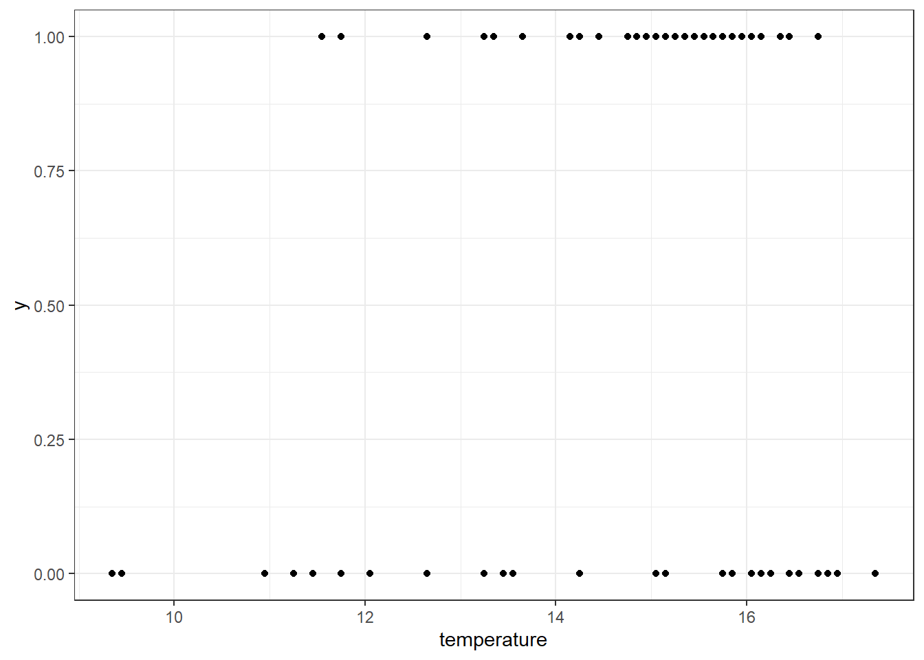
It seems like Redbreast Sunfish occurs more often at warmer sites, suggesting a potential positive relationship between air temperature (as a proxy for water temperature) and species presence.
6.2.4 Analysis
Visual inspection suggests a potential positive relationship between species occurrence and air temperature. But how do we know whether this pattern is real—or just due to chance? This is where statistical analysis becomes essential: it allows us to assess whether the observed relationship is unlikely to have occurred by random chance. While this book does not provide a comprehensive introduction to statistical theory, we will use the Generalized Linear Model (GLM) framework to analyze our dataset. Specifically, we will fit a Binomial regression model5 to evaluate the statistical influence of air temperature on the distribution of Redbreast Sunfish.
(m <- glm(y ~ temperature,
          data = df_rbs_tmp,
          family = "binomial"))
##
## Call: glm(formula = y ~ temperature, family = "binomial", data = df_rbs_tmp)
##
## Coefficients:
## (Intercept) temperature
## -5.8651 0.4583
##
## Degrees of Freedom: 121 Total (i.e. Null); 120 Residual
## Null Deviance: 142.4
## Residual Deviance: 130.6 AIC: 134.6The code glm(y ~ temperature, data = df_rbs_tmp, family = "binomial") fits a GLM to the data to examine the relationship between air temperature and the occurrence of Redbreast Sunfish.
In this model, y is a binary response variable indicating species presence (1) or absence (0), while temperature is the explanatory variable.
The data argument specifies the dataset being used (df_rbs_tmp), and the model formula (y ~ temperature) defines how the response depends on the predictor.
By setting family = "binomial", the model assumes that the response variable follows a binomial distribution, which is appropriate for binary outcomes.
This results in a logistic regression, where the model estimates the log-odds of species occurrence as a linear function of temperature.
The coefficients obtained from this model help us determine whether temperature has a statistically significant influence on species presence, beyond what we might expect from random variation alone.
The summary() function provides deeper insights:
summary(m)##
## Call:
## glm(formula = y ~ temperature, family = "binomial", data = df_rbs_tmp)
##
## Coefficients:
## Estimate Std. Error z value Pr(>|z|)
## (Intercept) -5.8651 2.1241 -2.761 0.00576 **
## temperature 0.4583 0.1417 3.234 0.00122 **
## ---
## Signif. codes: 0 '***' 0.001 '**' 0.01 '*' 0.05 '.' 0.1 ' ' 1
##
## (Dispersion parameter for binomial family taken to be 1)
##
## Null deviance: 142.43 on 121 degrees of freedom
## Residual deviance: 130.63 on 120 degrees of freedom
## AIC: 134.63
##
## Number of Fisher Scoring iterations: 4This output summarizes the results of a logistic regression assessing the effect of air temperature on the occurrence of Redbreast Sunfish.
The model includes an intercept and one predictor, temperature.
The intercept estimate is -5.8651, representing the log-odds of occurrence when temperature is zero (which may be outside the actual data range, so it’s not always biologically interpretable).
The coefficient for temperature is 0.4583, meaning that for each 1-unit increase in air temperature, the log-odds of species presence increase by 0.4583.
This translates to a higher probability of observing the species at warmer sites.
Both coefficients are statistically significant, with p-values well below 0.01 (0.00576 for the intercept and 0.00122 for temperature), indicating that the effect of temperature is unlikely due to random chance.
In this simplified case, we can easily visualize the model predictions using ggeffects::ggpredict():
df_pred <- ggpredict(m,
                     terms = "temperature [all]")

ggplot() +
  geom_point(data = df_rbs_tmp,
             aes(x = temperature,
                 y = y)) +
  geom_line(data = df_pred,
            aes(x = x,
                y = predicted)) +
  geom_ribbon(data = df_pred,
              aes(x = x,
                  ymin = conf.low,
                  ymax = conf.high),
              fill = "grey",
              alpha = 0.2) +
  labs(x = "Air temperature",
       y = "Probability of occurrence") +
  theme_bw()
This code generates a plot showing the predicted relationship between air temperature and the probability of Redbreast Sunfish occurrence, based on a logistic regression model.
The function ggpredict() is used with the argument terms = "temperature [all]", which computes predictions for every observed value of temperature in the dataset, ensuring a smooth and data-aligned prediction curve.
In the plot, each point represents an observation from the original dataset (df_rbs_tmp), showing where the species was present (y = 1) or absent (y = 0).
The black line shows the model-predicted probability of occurrence across the temperature gradient, while the shaded ribbon represents the 95% confidence interval around the prediction.
This result aligns well with ecological expectations—Redbreast Sunfish is a warm-water species known to prefer higher temperatures. The positive and statistically significant effect of air temperature on species occurrence supports this ecological knowledge. In other words, the statistical model confirms that Redbreast Sunfish are more likely to be found at warmer sites, validating the anticipated distributional response to air temperature.