14 Generalized Linear Model
One of the key assumptions in the Linear Model framework is Normality – that the error term follows a normal distribution (Chapter 13). However, this assumption frequently leads to situations where models predict unrealistic values for a response variable. In this chapter, I will introduce the Generalized Linear Model (GLM) framework, which enables more flexible modeling.
Key words: link function
14.1 Count Data
14.1.1 Plant Density
Recall our data set of garden plant counts (Chapter 9):
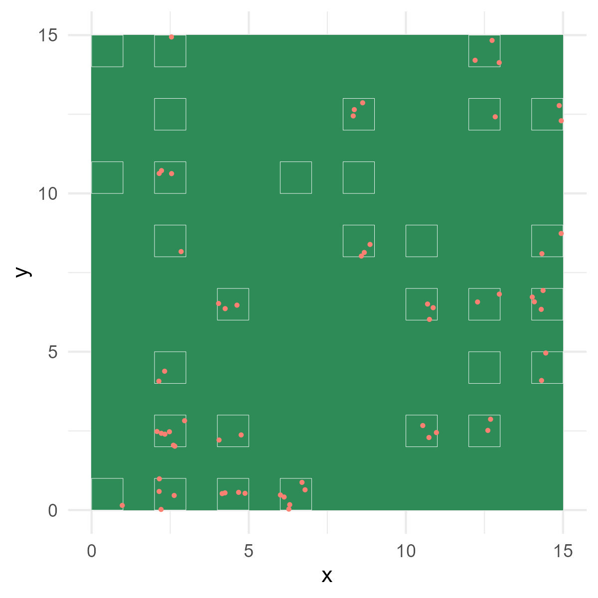
Figure 14.1: Garden view with sampling plots. White squares represent plots. Red dots indicate plant individuals counted.
## # A tibble: 30 × 3
##     plot count nitrate
##    <dbl> <dbl>   <dbl>
##  1     1     3    31.3
##  2     2     1    27.4
##  3     3     4    31.9
##  4     4     1    30.1
##  5     5     4    29.8
##  6     6     1    30.4
##  7     7     2    32
##  8     8     0    18.3
##  9     9     2    31.7
## 10    10     2    34
## # ℹ 20 more rows
The variable of plant count had the following characteristics:
The possible values are discrete (count data) since we are counting the number of plant individuals in each plot.
The possible values are always positive, as counts cannot be negative.
The distribution appears to be non-symmetric around the sample mean.
What happens if we apply a simple linear model that assumes a Normal distribution? Let me model the plant count as a function of nitrate as follows:
\[ \begin{aligned} y_i &\sim \text{Normal}(\mu_i, \sigma^2)\\ \mu_i &= \alpha + \beta~\text{nitrate}_i \end{aligned} \]
##
## Call:
## lm(formula = count ~ nitrate, data = df_count)
##
## Residuals:
##     Min      1Q  Median      3Q     Max
## -1.2782 -0.6020 -0.1625  0.5094  3.1272
##
## Coefficients:
##             Estimate Std. Error t value Pr(>|t|)
## (Intercept) -4.17690    1.20371  -3.470   0.0017 **
## nitrate      0.21234    0.04068   5.219 1.52e-05 ***
## ---
## Signif. codes:  0 '***' 0.001 '**' 0.01 '*' 0.05 '.' 0.1 ' ' 1
##
## Residual standard error: 0.9975 on 28 degrees of freedom
## Multiple R-squared:  0.4931, Adjusted R-squared:  0.475
## F-statistic: 27.24 on 1 and 28 DF,  p-value: 1.523e-05
This seems satisfactory, but an anomalous behavior occurs during the plotting process on the figure. Plot the data and the predicted values together.
# extract estimates
alpha <- coef(m_normal)[1] # intercept
beta <- coef(m_normal)[2] # slope

df_count %>%
  ggplot(aes(x = nitrate,
             y = count)) +
  geom_point() +
  geom_abline(intercept = alpha,
              slope = beta)
The intersection of the predicted line with the x-axis suggests the presence of negative predicted values for plant counts. However, it is logically implausible for plant counts to be negative.
This occurrence stems from the nature of the model employed.
- In the Linear Model with a Normal error distribution, we allow the mean to encompass a wide range of values, including negative values.
- Even when the mean predicted values do not intersect the x-axis, we consider the possibility of observations taking negative values, as dictated by the nature of a Normal distribution (\(\mu_i + \varepsilon_i\) can be negative even when \(\mu_i > 0\)), which in reality can never occur.
14.1.2 Poisson Model
One possible approach is to consider the assumption that the error term follows a Poisson distribution. For the purpose of this discussion, let’s assume that a model based on the Poisson distribution is appropriate. Unlike a Normal distribution, the Poisson distribution generates only non-negative discrete values, which makes it a suitable fit for the plant count variable. To incorporate this, we can make the following modifications to the model:
\[ \begin{aligned} y_i &\sim \text{Poisson}(\lambda_i)\\ \log\lambda_i &= \alpha + \beta~\text{nitrate}_i \end{aligned} \]
These changes are crucial:
- The plant count, denoted as \(y_i\), is now assumed to follow a Poisson distribution with parameter \(\lambda_i\). This ensures that negative values of \(y_i\) are not possible (i.e., \(\Pr(y_i < 0) = 0\)).
- The mean \(\lambda_i\) is log-transformed when expressing it as a function of nitrate. Given that the mean of a Poisson distribution cannot be negative, we must restrict the range of \(\lambda_i\) to positive values. The log-transformation guarantees positivity of \(\lambda_i\) (\(\lambda_i = \exp(\alpha + \beta~\text{nitrate}_i)\)) irrespective of the values of \(\alpha\), \(\beta\), and \(\text{nitrate}_i\).
The implementation of the Poisson model is quite simple. In the following example, we will use the function glm():
m_pois <- glm(count ~ nitrate,
              data = df_count,
              family = "poisson")
The major difference from lm() is the argument family = "poisson". This argument specifies the probability distribution to be used; in this example, I used a Poisson distribution to model count data. However, in looking at estimates…
summary(m_pois)##
## Call:
## glm(formula = count ~ nitrate, family = "poisson", data = df_count)
##
## Coefficients:
## Estimate Std. Error z value Pr(>|z|)
## (Intercept) -4.70258 1.58317 -2.970 0.002974 **
## nitrate 0.17751 0.05035 3.525 0.000423 ***
## ---
## Signif. codes: 0 '***' 0.001 '**' 0.01 '*' 0.05 '.' 0.1 ' ' 1
##
## (Dispersion parameter for poisson family taken to be 1)
##
## Null deviance: 32.015 on 29 degrees of freedom
## Residual deviance: 13.628 on 28 degrees of freedom
## AIC: 86.661
##
## Number of Fisher Scoring iterations: 5The estimated intercept is still negative…what’s wrong? No sweat, we estimated these parameters in a log scale; this result translates into:
\[ \lambda_i = \exp(-4.05 + 0.17~\text{nitrate}_i) \]
Therefore, even when the intercept is estimated to be negative, the mean \(\lambda_i\) is guaranteed to be non-negative.
Another important difference from lm() is that the test-statistic is no long the t-statistic – instead, glm() reports the z-statistic. However, the z-statistic is very similar to the t-statistic, defined as \(z=\frac{\hat{\theta} - \theta_0}{\text{SE}(\hat{\theta})}\) (\(\hat{\theta} \in \{\hat{\alpha}, \hat{\beta}\}\), \(\theta_0 = 0\)). Therefore, you can reproduce the z-statistic by dividing the parameter estimates (\(\hat{\alpha}\) and \(\hat{\beta}\)) by their standard errors:
# parameter estimates and their SEs
theta <- coef(m_pois)
se <- sqrt(diag(vcov(m_pois)))
z_value <- theta / se

print(z_value)
## (Intercept) nitrate
## -2.970364 3.525377We call this statistic “z-statistic” as it is known to follow the z-distribution (also known as the standardized Normal distribution \(\text{Normal}(0, 1)\)), as opposed to the Student’s t-distribution. The reported p-value (Pr(>|z|)) is estimated under this assumption, which can be seen as follows.
# estimate Pr(>|z|) using a standardized normal distribution
p_value <- (1 - pnorm(abs(z_value), mean = 0, sd = 1)) * 2
print(p_value)
## (Intercept) nitrate
## 0.0029744722 0.0004228806Notice that these p-values are not identical to the output from the Normal model – therefore, the choice of the probability distribution critically affects the results of statistical analysis, and often times, qualitatively (not in this particular example though).
Visualization provides the convincing difference between the Normal and Poisson models (Figure 14.2).
# make predictions
df_pred <- tibble(nitrate = seq(min(df_count$nitrate),
                                max(df_count$nitrate),
                                length = 100))

# y_pois is exponentiated because predict() returns values in log-scale
y_normal <- predict(m_normal, newdata = df_pred)
y_pois <- predict(m_pois, newdata = df_pred) %>% exp()

df_pred <- df_pred %>%
  mutate(y_normal,
         y_pois)

# figure
df_count %>%
  ggplot(aes(x = nitrate,
             y = count)) +
  geom_point() +
  geom_line(data = df_pred,
            aes(y = y_normal),
            linetype = "dashed") +
  geom_line(data = df_pred,
            aes(y = y_pois),
            color = "salmon")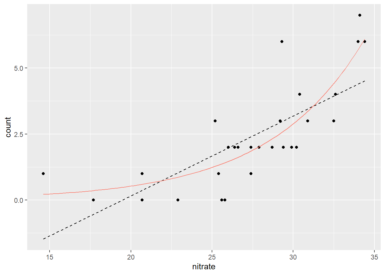
Figure 14.2: Comparison of the predicted values between Normal (broken, black) and Poisson models (solid, red).
Clearly, the Poisson model does a better job.
14.2 Proportional Data
14.2.1 Mussel Egg Fertilization
There is another type of data for which a Normal distribution is not suitable - proportional data. Let’s consider an example dataset where an investigation was conducted on the number of fertilized eggs out of 30 eggs examined for 100 female freshwater mussels. You can download the dataset here.
Male freshwater mussels release sperm into the water, which is then drawn into female mussels downstream. Considering the nature of the fertilization process, female mussels are expected to have a higher probability of fertilization when they are surrounded by a greater number of males. To explore this relationship, let’s load the data into R and visualize it.
## # A tibble: 100 × 4
##    ind_id n_fertilized n_examined density
##     <dbl>        <dbl>      <dbl>   <dbl>
##  1      1            0         30       6
##  2      2           17         30      15
##  3      3           21         30      15
##  4      4            3         30       9
##  5      5            1         30       9
##  6      6            7         30      11
##  7      7            2         30       9
##  8      8            0         30       2
##  9      9            1         30       9
## 10     10            0         30       7
## # ℹ 90 more rows
This data frame contains variables such as ind_id (mussel individual ID), n_fertilized (number of fertilized eggs), n_examined (number of eggs examined), and density (number of mussels in a 1 m\(^2\) quadrat). To visualize the relationship between the proportion of eggs fertilized and the density gradient, plot the proportion of fertilized eggs against the density gradient (Figure 14.3).
# calculate the proportion of fertilized eggs
df_mussel <- df_mussel %>%
  mutate(prop_fert = n_fertilized / n_examined)

# plot
df_mussel %>%
  ggplot(aes(x = density,
             y = prop_fert)) +
  geom_point() +
  labs(y = "Proportion of eggs fertilized",
       x = "Mussel density")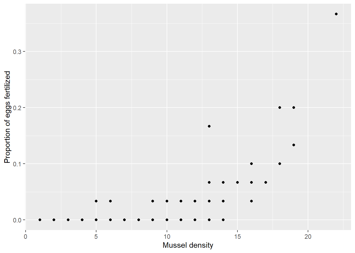
Figure 14.3: Relationship between the proportion of fertilized eggs and mussel density in the surround.
In this example, the response variable, which represents the number of eggs fertilized, possesses the following characteristics:
Discreteness: The variable takes on discrete values rather than continuous ones.
Upper limit: The number of eggs fertilized is bounded by an upper limit (in this case, 30).
The discrete nature of the variable might initially lead one to consider the Poisson distribution as a potential candidate. However, due to the presence of an upper limit where the number of fertilized eggs cannot exceed the number of eggs examined, the Poisson distribution is not a suitable option.
14.2.2 Binomial Model
A Binomial distribution is a natural and appropriate choice for modeling this variable. The Binomial distribution is characterized by two parameters: the number of trials (\(N\)) and the probability of success (\(p\)). Each trial has a certain probability of success, and the outcome of each trial is either assigned a value of 1 (indicating success) or 0 (indicating failure). In the given example, we can consider the “fertilization” as a successful outcome among the 30 trials. Consequently, the number of eggs fertilized (\(y_i\)) for each individual mussel (\(i\)) can be described as:
\[ y_i \sim \text{Binomial}(N_i, p_i) \]
This formulation adequately captures the nature of the response variable, as the outcome of the Binomial distribution is constrained within the range of \(0\) to \(N_i\), aligning with the upper limit imposed by the number of examined eggs.
Our prediction was that the fertilization probability \(p_i\) would increase with increasing mussel’s density – how do we relate \(p_i\) to mussel density? The value of \(p_i\) must be constrained within a range of \(0.0-1.0\) because it is a “probability.” Given this, the log-transformation, which we used in the Poisson model, is not a suitable choice. Instead, we can use a logit-transformation to convert the linear formula to fall within a range of \(0.0 - 1.0\).
\[ \begin{aligned} y_i &\sim \text{Binomial}(N_i, p_i)\\ \log(\frac{p_i}{1-p_i}) &= \alpha + \beta~\text{density}_i \end{aligned} \]
The logit transformation, represented as \(\log\left(\frac{p_i}{1-p_i}\right)\), guarantees that the values of \(p_i\) are confined within the range of 0.0 to 1.0. This relationship is expressed by the following equation:
\[ p_i = \frac{\exp(\alpha + \beta~\text{density}_i)}{1 + \exp(\alpha + \beta~\text{density}_i)} \]
A straightforward coding can verify this.
# x: produce 100 numbers from -100 to 100 (assume logit scale)
# y: convert with inverse-logit transformation (ordinary scale)
df_test <- tibble(logit_x = seq(-10, 10, length = 100),
                  x = exp(logit_x) / (1 + exp(logit_x)))

df_test %>%
  ggplot(aes(x = logit_x,
             y = x)) +
  geom_point() +
  geom_line() +
  labs(y = "x",
       x = "logit(x)")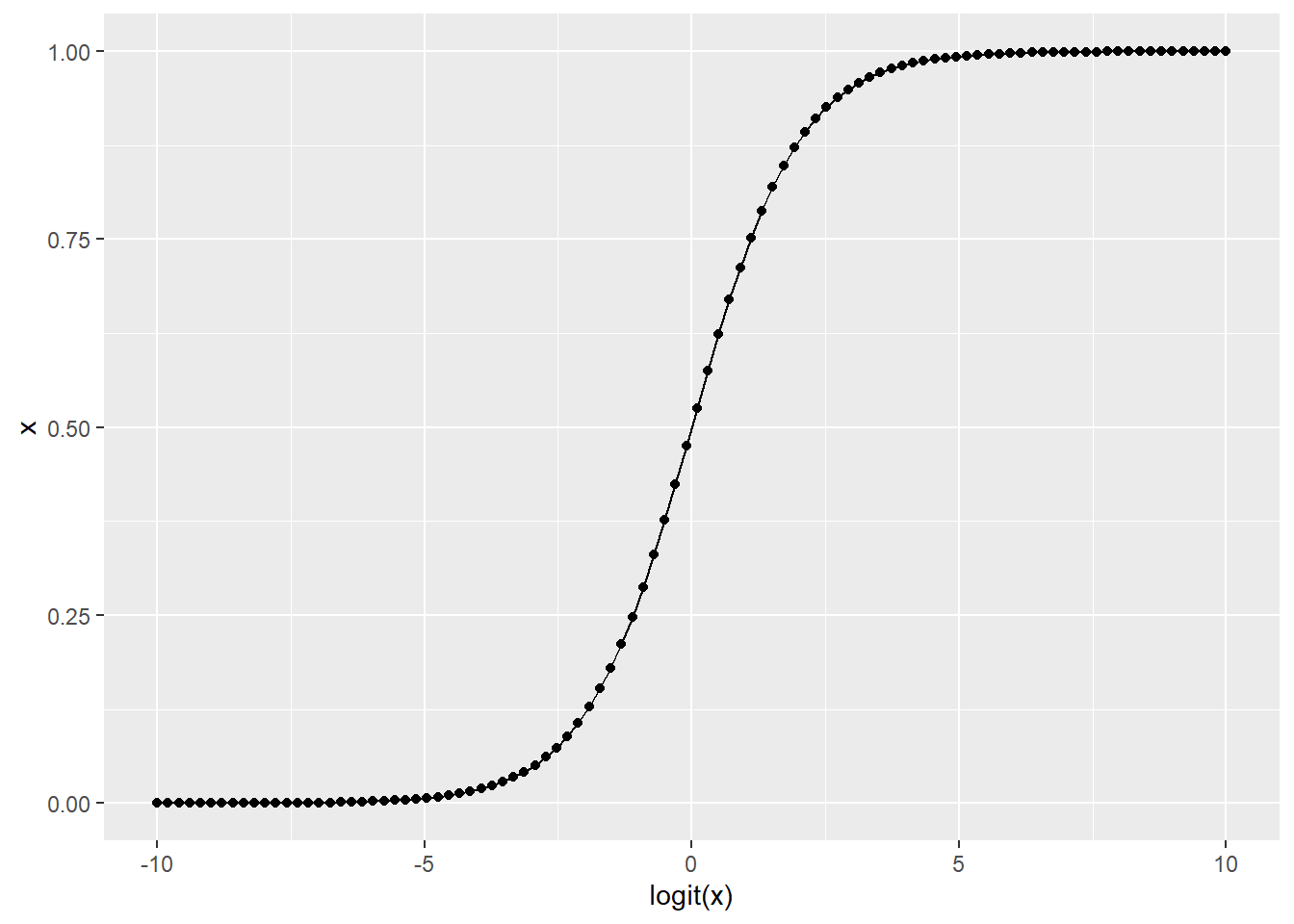
Figure 14.4: Logit-transformation ensures that the transformed variable to fall in the range of zero to one.
The glm() function can be used to implement this modeling approach. However, certain modifications need to be made to the response variable in order to ensure compatibility with the binomial distribution.
m_binom <- glm(cbind(n_fertilized, n_examined - n_fertilized) ~ density,
               data = df_mussel,
               family = "binomial")
In contrast to the Normal or Poisson models, the response variable was encoded using the cbind(n_fertilized, n_examined - n_fertilized) function. The cbind() function combines the number of successes (fertilized) and failures (not fertilized) into a single matrix. This approach allows for modeling the data using the binomial distribution, taking into account both the successes and the total number of trials within each observation.
##      [,1] [,2]
## [1,]    0   30
## [2,]   17   13
## [3,]   21    9
## [4,]    3   27
## [5,]    1   29
## [6,]    7   23
Similar to the previous examples, the summary() function provides estimates of the model parameters. By applying the summary() function to the fitted model, you can obtain information such as coefficient estimates, standard errors, p-values, and other relevant statistics.
summary(m_binom)##
## Call:
## glm(formula = cbind(n_fertilized, n_examined - n_fertilized) ~
## density, family = "binomial", data = df_mussel)
##
## Coefficients:
## Estimate Std. Error z value Pr(>|z|)
## (Intercept) -7.85097 0.27150 -28.92 <2e-16 ***
## density 0.58219 0.02142 27.18 <2e-16 ***
## ---
## Signif. codes: 0 '***' 0.001 '**' 0.01 '*' 0.05 '.' 0.1 ' ' 1
##
## (Dispersion parameter for binomial family taken to be 1)
##
## Null deviance: 1676.42 on 99 degrees of freedom
## Residual deviance: 104.66 on 98 degrees of freedom
## AIC: 317.64
##
## Number of Fisher Scoring iterations: 5This result translates into:
\[ \begin{aligned} y_i &\sim \text{Binomial}(N_i, p_i)\\ \log(\frac{p_i}{1 - p_i}) &= -8.06 + 0.34~\text{density}_i \end{aligned} \]
To make predictions, it is necessary to back-transform the predicted fertilization probability since it is estimated on a logit scale. The back-transformation will convert the predicted values back to the original probability scale (\(0.0-1.0\)).
# make prediction
df_pred <- tibble(density = seq(min(df_mussel$density),
                                max(df_mussel$density),
                                length = 100))

# y_binom is inv.logit-transformed because predict() returns values in logit-scale
y_binom <- predict(m_binom, newdata = df_pred) %>% boot::inv.logit()

df_pred <- df_pred %>%
  mutate(y_binom)
Draw on the figure (Figure 14.5).
df_mussel %>%
  ggplot(aes(x = density,
             y = prop_fert)) +
  geom_point() +
  geom_line(data = df_pred,
            aes(y = y_binom)) +
  labs(y = "Proportion of eggs fertilized",
       x = "Mussel density")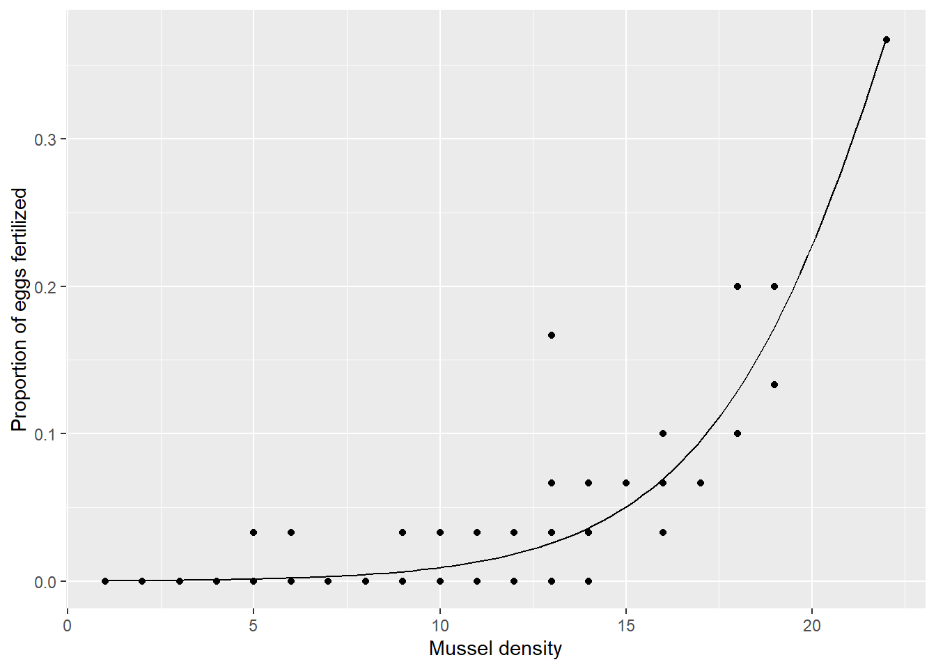
Figure 14.5: Prediction by the Binomial model.
Perfect.
14.3 The GLM Framework
These models, including those assuming a Normal distribution, fall into the category of the Generalized Linear Model (GLM) framework. The framework follows a common structure:
\[ \begin{aligned} y_i &\sim \text{D}(\Theta)\\ \text{Link}(\mbox{E}(y_i)) &= \alpha + \sum_k \beta_k x_{k, i} \end{aligned} \]
In this structure, \(\Theta\) represents a parameter vector of the probability distribution, while \(\text{D}(\cdot)\) and \(\text{Link}(\cdot)\) denote the chosen probability distribution and its associated link function, respectively. For example, if we select a Poisson distribution as \(\text{D}(\cdot)\), then the corresponding \(\text{Link}(\cdot)\) function is the natural logarithm (log) (see Section 14.1.2). The expected value \(\mbox{E}(y_i)\) is expressed as a function of parameter(s) of the probability distribution \(f(\Theta)\), which is related to the explanatory variables \(x\). For instance, in Normal and Poisson models, we model the mean, while in the Binomial model, we model the success probability. In certain distributions, \(f(\Theta)\) may be a function of multiple parameters.
The GLM framework differs from the Linear Model framework by offering greater flexibility in the choice of probability distribution, achieved through the introduction of the Link function. This function allows us to constrain the modeled parameter within a specific range. As non-normal distributions are common in natural phenomena, this framework plays a critical role in modern statistical analysis.
However, how do we determine the appropriate probability distribution? While there is no single correct answer to this question, there are clear factors to consider—specifically, the characteristics of the response variable. The following criteria can be particularly helpful:
- Is the variable discrete?
- Is there an upper bound?
- Is the sample variance far greater than the mean?
To assist you in selecting an appropriate probability distribution for modeling, I have provided a concise decision tree graph. Please note that the choices presented are frequently encountered in ecological modeling, rather than an exhaustive list of probability distributions (see Table 14.1). The full list of probability distributions can be found here (Wikipedia page)
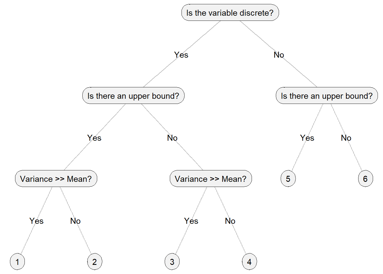
Figure 14.6: Tree chart on how to choose a probability distribution in GLM analysis.
| # | Distribution | Support | R |
|---|---|---|---|
| 1 | Beta-binomial | [0, N] | glmmTMB::glmmTMB() |
| 2 | Binomial | [0, N] |
glm(), glmmTMB::glmmTMB()
|
| 3 | Negative binomial | \(\ge 0\) |
MASS::glm.nb(), glmmTMB::glmmTMB()
|
| 4 | Poisson | \(\ge 0\) |
glm(), glmmTMB::glmmTMB()
|
| 5 | Beta | (0, 1) | glmmTMB::glmmTMB() |
| 6 | Normal | \(-\infty\) to \(\infty\) |
lm(), glm(), glmmTMB::glmmTMB()
|
14.4 Laboratory
14.4.1 GLM exercise
-
A publicly available stream fish distribution dataset can be accessed from an online repository:
url <- "https://raw.githubusercontent.com/aterui/public-proj_fish-richness-shubuto/master/data/data_vpart.csv"
df_fish <- read_csv(url)
The dataset comprises information on the number of species found at each site (
n_sp) and several associated environmental variables, including distance to the sea (distance), catchment area (cat_area), and environmental heterogeneity (hull_area). These environmental variables are factors that are known to influence fish distributions. To analyze this dataset, develop a Generalized Linear Model (GLM) as follows:- Use fish species richness
n_spas a response variable of the model with an appropriate probability distribution (family). Identify which predictor variable(s) significantly influence the response variable.
- Use fish species richness
-
The
mtcarsdataset contains information about 32 car models, including their performance and design characteristics. The variableamindicates the type of transmission, where0 = automaticand1 = manual.Using this dataset, develop a GLM to explore:
Which variables significantly influence the probability that a car has a manual transmission? Choose an appropriate probability distribution (
family). Consider including the following predictors: miles per gallon (mpg), horsepower (hp), and weight (wt).Develop the same GLM but with a normal distribution (
family = "gaussian"). Compare the results to the model with an appropriate probability distribution.
14.4.2 Effect size
Often, we are interested in comparing the effect sizes of different explanatory variables. However, if we use raw environmental values, regression coefficients are not directly comparable due to their differing units. Recall that regression coefficients represent the increment of \(y\) per unit increase of \(x\). To facilitate comparison, we standardize the explanatory variables by subtracting their means and dividing them by their standard deviations:
\[ \mbox{E}(y) = \alpha + \beta x \rightarrow \mbox{E}(y) = \alpha' + \beta' \frac{(x - \mu_x)}{\sigma_x} \]
Here, \(\alpha'\) and \(\beta'\) represent the intercept and slope after standardizing \(x\), respectively.
The function
scale()will perform standardization. Create columns of standardizeddistance(std_dist),cat_area(std_cat), andhull_area(std_hull).Perform a GLM analysis of fish species richness with the standardized variables, and identify the most influential variable among them in terms of effect size.
14.4.3 Offset term
-
The Poisson distribution (and other distributions used for modeling count data) assumes that all observations are collected under comparable sampling efforts. In practice, however, survey data often differ in effort — for example, some counts may come from surveys conducted over longer search times or larger areas. To see this issue, copy and paste the following code:
url <- "https://raw.githubusercontent.com/aterui/biostats/master/data_raw/data_offset.csv"
df_offset <- read_csv(url)
Using
df_offset, perform the following:- Plot the relationship between
countandnitrate. - Plot the relationship between
countandarea. - Plot the relationship between
count/areaandnitrate.
- Plot the relationship between
-
Directly comparing such counts would be misleading because higher effort naturally increases the expected number of detections. One might consider dividing the response variable by effort to standardize it, but doing so changes the outcome from a discrete count to a continuous rate, violating the assumptions of count models. Confirm the following code returns numerous wranings – this is because
densityis not a discrete variable:df_offset <- df_offset %>% mutate(density = count / area) glm(density ~ nitrate, data = df_offset, family = "poisson")A better approach is to incorporate sampling effort as an offset term in
glm(), which allows the model to account for differences in effort while preserving the count nature of the response variable. Perform the following exercise:- Develop a GLM with the response variable
countand the predictornitrate. - Develop a GLM with the response variable
count, the predictornitrate, and the offset termoffset(log(area))(~ nitrate + offset(log(area))will work). - Compare the results of the two models.
- Develop a GLM with the response variable
14.4.4 Overdispersion
Copy and paste the following code:
url <- "https://raw.githubusercontent.com/aterui/biostats/master/data_raw/data_tadpole.csv"
df_tadpole <- read_csv(url)
This dataset contains the data of tadpole counts (tadpole), aquatic vegetation cover (aqveg), and pond permanence (the number of days persist; permanence).
Plot the relationships between (a)
tadpoleandaqvegand (b)tadpoleandpermanence.Discuss in a group that which variable may have significant influence.
Develop a GLM (choose an appropriate distribution) explaining
tadpolewithaqvegandpermanence.