mcsim

Basic usage

mcsim() simulates metacommunity dynamics in a given landscape. Community dynamics are modeled based on the Beverton-Holt function. Although this function is designed to be compatible with brnet(), users can provide their distance matrix to simulate dynamics in any landscape. The key arguments are the number of habitat patches (n_patch) and the number of species in a metacommunity (n_species). Metacommunity dynamics are simulated through (1) local dynamics (population growth and competition among species), (2) immigration, and (3) emigration.

The function returns:

df_dynamics data frame containing simulated metacommunity dynamics*.
- timestep: time-step.
- patch_id: patch ID.
- mean_env: mean environmental condition at each patch.
- env: environmental condition at patch x and time-step t.
- carrying_capacity: carrying capacity at each patch.
- species: species ID.
- niche_optim: optimal environmental value for species i.
- r_xt: reproductive number of species i at patch x and time-step t.
- abundance: abundance of species i at patch x.
df_species data frame containing species attributes.
- species: species ID.
- mean_abundance: mean abundance (arithmetic) of species i across sites and time-steps.
- r0: maximum reproductive number of species i.
- niche_optim: optimal environmental value for species i.
- sd_niche_width: niche width for species i.
- p_dispersal: dispersal probability of species i.
df_patch data frame containing patch attributes.
- patch_id: patch ID.
- alpha_div: alpha diversity averaged across time-steps.
- mean_env: mean environmental condition at each patch.
- carrying_capacity: carrying capacity at each patch.
- disturbance: disturbance-induced mortality at each patch.
df_diversity data frame containing diversity metrics (α, β, and γ).
distance_matrix distance matrix used in the simulation.
interaction_matrix species interaction matrix, in which species X (column) influences species Y (row).

*NOTE: The warm-up and burn-in periods will not be included in return values.

Quick start

The following script simulates metacommunity dynamics with n_patch = 5 and n_species = 5. By default, mcsim() simulates metacommunity dynamics with 200 warm-up (initialization with species introductions: n_warmup), 200 burn-in (burn-in period with no species introductions: n_burnin), and 1000 time-steps for records (n_timestep).

mc <- mcsim(n_patch = 5, n_species = 5)

Users can visualize the simulated dynamics using plot = TRUE, which will show five sample patches and species that are randomly chosen:

mc <- mcsim(n_patch = 5, n_species = 5, plot = TRUE)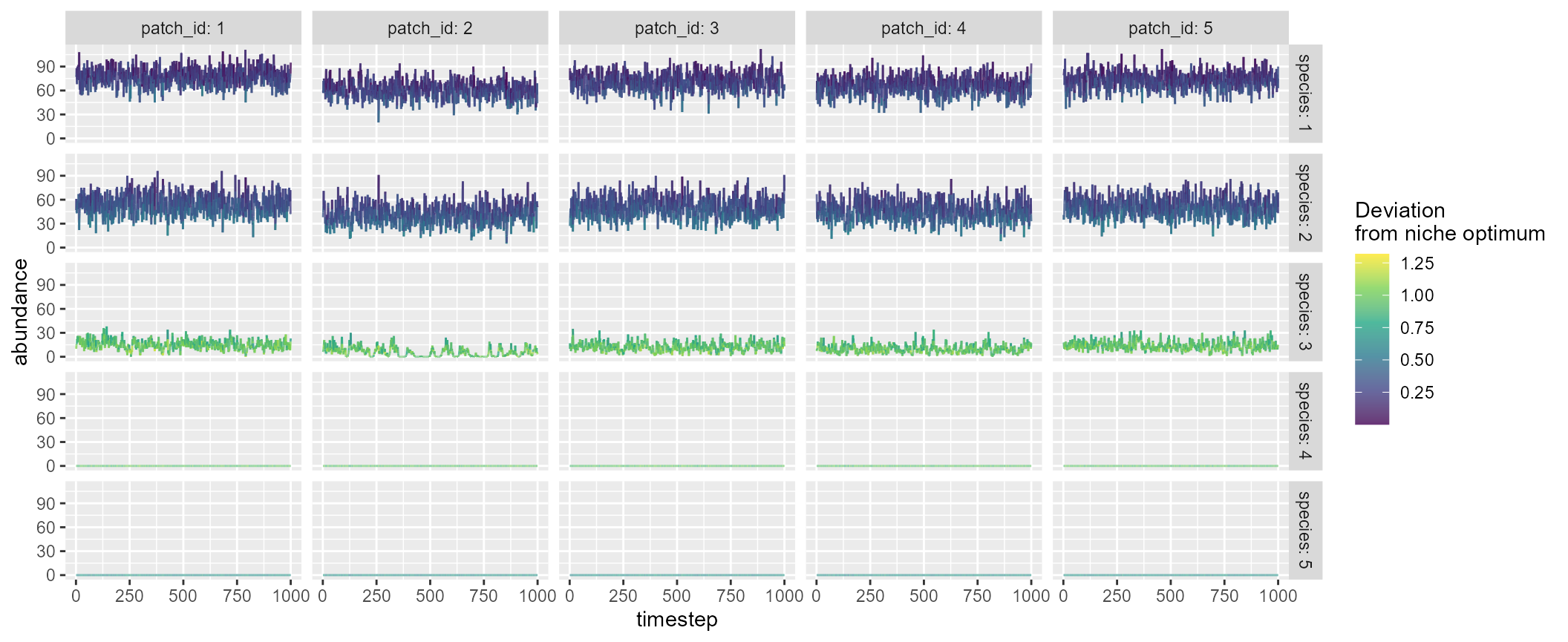

A named list of return values:

mc
#> $df_dynamics
#> # A tibble: 25,000 × 9
#>    timestep patch_id mean_env      env carrying_capacity species niche_optim
#>       <dbl>    <dbl>    <dbl>    <dbl>             <dbl>   <dbl>       <dbl>
#>  1        1        1        0 -0.120                 100       1       0.239
#>  2        1        1        0 -0.120                 100       2      -0.344
#>  3        1        1        0 -0.120                 100       3       0.947
#>  4        1        1        0 -0.120                 100       4       0.937
#>  5        1        1        0 -0.120                 100       5       0.665
#>  6        1        2        0  0.00735               100       1       0.239
#>  7        1        2        0  0.00735               100       2      -0.344
#>  8        1        2        0  0.00735               100       3       0.947
#>  9        1        2        0  0.00735               100       4       0.937
#> 10        1        2        0  0.00735               100       5       0.665
#> # ℹ 24,990 more rows
#> # ℹ 2 more variables: r_xt <dbl>, abundance <dbl>
#> 
#> $df_species
#> # A tibble: 5 × 6
#>   species mean_abundance    r0 niche_optim sd_niche_width p_dispersal
#>     <dbl>          <dbl> <dbl>       <dbl>          <dbl>       <dbl>
#> 1       1           69.5     4       0.239          0.461         0.1
#> 2       2           47.8     4      -0.344          0.388         0.1
#> 3       3           11.3     4       0.947          0.786         0.1
#> 4       4            0       4       0.937          0.115         0.1
#> 5       5            0       4       0.665          0.412         0.1
#> 
#> $df_patch
#> # A tibble: 5 × 5
#>   patch_id alpha_div mean_env carrying_capacity disturbance
#>      <dbl>     <dbl>    <dbl>             <dbl>       <dbl>
#> 1        1      3.00        0               100           0
#> 2        2      2.72        0               100           0
#> 3        3      3           0               100           0
#> 4        4      3.00        0               100           0
#> 5        5      3           0               100           0
#> 
#> $df_diversity
#> # A tibble: 1 × 3
#>   alpha_div beta_div gamma_div
#>       <dbl>    <dbl>     <dbl>
#> 1      2.94     1.02         3
#> 
#> $df_xy_coord
#> # A tibble: 5 × 2
#>   x_coord y_coord
#>     <dbl>   <dbl>
#> 1   5.57     7.57
#> 2   8.82     3.05
#> 3   3.89     5.14
#> 4   0.980    6.86
#> 5   4.33     9.57
#> 
#> $distance_matrix
#>          1        2        3        4        5
#> 1 0.000000 5.565821 2.958187 4.645296 2.353877
#> 2 5.565821 0.000000 5.353711 8.714434 7.915863
#> 3 2.958187 5.353711 0.000000 3.379341 4.455747
#> 4 4.645296 8.714434 3.379341 0.000000 4.310462
#> 5 2.353877 7.915863 4.455747 4.310462 0.000000
#> 
#> $interaction_matrix
#>      [,1] [,2] [,3] [,4] [,5]
#> [1,]    1    0    0    0    0
#> [2,]    0    1    0    0    0
#> [3,]    0    0    1    0    0
#> [4,]    0    0    0    1    0
#> [5,]    0    0    0    0    1

Custom: `brnet()` + `mcsim()`

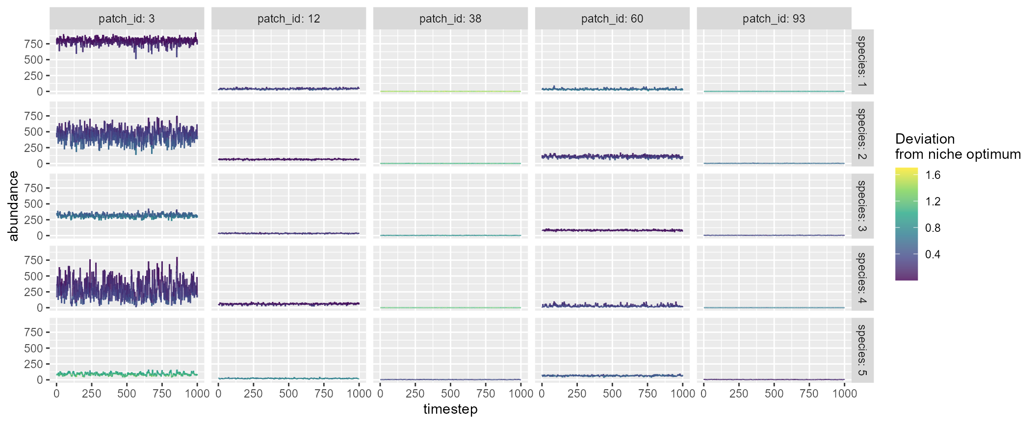
brnet() outputs are compatible with mcsim(). For example, df_patch$environment, df_patch$n_patch_upstream, and df_patch$distance_matrix may be used to inform arguments in mcsim():

patch <- 100
net <- brnet(n_patch = patch,
             p_branch = 0.5)

mc <- with(net,
           mcsim(n_patch = patch,
                 n_species = 5,
                 mean_env = df_patch$environment,
                 carrying_capacity = df_patch$n_patch_upstream * 10,
                 distance_matrix = distance_matrix,
                 plot = TRUE)
           )

Custom: parameter detail

Users can tweak (1) species attributes, (2) competition, (3) patch attributes, and (4) landscape structure.

Species attributes

Arguments: r0, niche_optim OR min_optim and max_optim, sd_niche_width OR min_niche_width and max_niche_width, niche_cost, p_dispersal , zeta

Species attributes are determined based on the maximum reproductive rate r0, optimal environmental value niche_optim (or min_optim and max_optim for random generation of niche_optim), niche width sd_niche_width (or min_niche_width and max_niche_width for random generation of sd_niche_width) and dispersal probability p_dispersal (see Model description for details).

For optimal environmental values (niche optimum), the function by default assigns random values to species as: $\mu_i \sim \mbox{Unif}(\mu_{min}, \mu_{max})$ , where users can set values of $\mu_{min}$ and $\mu_{max}$ using min_optim and max_optim arguments (default: min_optim = -1 and max_optim = 1). Alternatively, users may specify species niche optimums using the argument niche_optim (scalar or vector). If a single value or a vector of niche_optim is provided, the function ignores min_optim and max_optim arguments.

Similarly, the function by default assigns random values of $\sigma_{niche}$ to species as: $\sigma_{niche,i} \sim \mbox{Unif}(\sigma_{niche,min}, \sigma_{niche,max})$ . Users can set values of $\sigma_{niche,min}$ and $\sigma_{niche,max}$ using min_niche_width and max_niche_width arguments (default: min_niche_width = 0.1 and max_niche_width = 1). If a single value or a vector of sd_niche_width is provided, the function ignores min_niche_width and max_niche_width arguments.

The argument niche_cost determines the cost of having wider niche. Smaller values imply greater costs of wider niche (i.e., decreased maximum reproductive rate; default: niche_cost = 1). To disable (no cost of wide niche), set niche_cost = Inf.

For other parameters, users may specify species attributes by giving a scalar (assume identical among species) or a vector of values whose length must be one or equal to n_species. Default values are r0 = 4, sd_niche_width = 1, and p_dispersal = 0.1.

The argument zeta determines the sensitivity to environmental pollutants as $\exp(-\zeta~impact)$ , which will be multiplied with the patch-specific population growth to represent negative impacts of pollutants. $impact$ represents the concentration of hypothetical environmental pollutants (see q in patch attributes). The parameter $\zeta$ determines the sensitivity to environmental pollutants, and larger values indicate greater species sensitivity. No pollutant effect if $\zeta = 0$ .

Competition

Arguments: interaction_type, alpha OR min_alpha and max_alpha

The argument interaction_type determines whether interaction coefficient alpha is a constant or random variable. If interaction_type = "constant", then the interaction coefficients $\alpha_{ij, i \ne j}$ for any pairs of species will be set as a constant alpha (i.e., off-diagonal elements of the interaction matrix). If interaction_type = "random", $\alpha_{ij, i \ne j}$ will be drawn from a uniform distribution as $\alpha_{ij, i \ne j} \sim \mbox{Unif}(\alpha_{min}, \alpha_{max})$ with corresponding arguments min_alpha and max_alpha. The argument alpha is ignored under the scenario of random interaction strength (i.e., interaction_type = "random"). Note that the diagonal elements of the interaction matrix ( $\alpha_{ii}$ ) are always 1.0 regardless of interaction_type, as alpha is the strength of interspecific competition relative to that of intraspecific competition (see Model description). By default, interaction_type = "constant" and alpha = 0.

Patch attributes

Arguments: carrying_capacity, mean_env, sd_env, spatial_env_cor, phi, p_disturb, i_disturb , impact

The arguments carrying_capacity (default: carrying_capacity = 100) and mean_env (default: mean_env = 0) determines mean environmental values of habitat patches, which can be a scalar (assume identical among patches) or a vector (length must be equal to n_patch).

The arguments sd_env (default: sd_env = 0.1), spatial_env_cor (default: spatial_env_cor = FALSE) and phi (default: phi = 1) determine spatio-temporal dynamics of environmental values. sd_env determines the magnitude of temporal environmental fluctuations. If spatial_env_cor = TRUE, the function models spatial autocorrelation of temporal environmental fluctuation based on a multi-variate normal distribution. The degree of spatial autocorrelation would be determined by phi, the parameter describing the strength of distance decay in spatial autocorrelation.

Users can also define disturbance probability (p_disturb) and mortality (i_disturb). When disturbance occurs, all habitat patches are reduced by i_disturb. i_disturb can be identical or different across habitat patches.

Lastly, the argument impact defines concentration of hypothetical environmental pollutants. The values will be converted as $\exp(-\zeta~impact)$ , which will be multiplied with the patch-specific population growth. Thus, a greater reduction factor will be applied as the value of $impact$ increases. The parameter $\zeta$ determines the sensitivity to environmental pollutants (see argument zeta in species attributes).

Landscape structure

Arguments: xy_coord OR distance_matrix, landscape_size, theta

These arguments define landscape structure. By default, the function produces a square-shaped landscape (landscape_size = 10 on a side) in which habitat patches are distributed randomly through a Poisson point process (i.e., x- and y-coordinates of patches are drawn from a uniform distribution). The parameter θ describes the shape of distance decay in species dispersal (see Model description) and determines patches’ structural connectivity (default: theta = 1). Users can define their landscape by providing either xy_coord or distance_matrix (landscape_size will be ignored if either of these arguments is provided). If xy_coord is provided (2-column data frame denoting x- and y-coordinates of patches, respectively; NULL by default), the function calculates the distance between patches based on coordinates. Alternatively, users may provide distance_matrix (the object must be matrix), which describes the distance between habitat patches. The argument distance_matrix overrides xy_coord.

Others

Arguments: n_warmup, n_burnin, n_timestep

The argument n_warmup is the period during which species introductions occur (default: n_warmup = 200). The initial number of individuals introduced follows a Poisson distribution with a mean of 0.5 and independent across space and time. This random introduction events occur multiple times over the n_warmup period, in which propagule_interval determines the timestep interval of the random introductions (default: propagule_interval = ceiling(n_warmup / 10)).

The argument n_burnin is the period that will be discarded as burn-in to remove the influence of initial values (default: n_burnin = 200). During the burn-in period, species introductions do not occur.

The argument n_timestep is the simulation peiord that is recorded in the return df_dynamics (default: n_timestep = 1000). As a result, with the default setting, the function simulates 1400 timesteps (n_warmup + n_burnin + n_timestep = 1400) but returns only the last 1000 timesteps as the resulting metacommunity dynamics. All the derived statistics (e.g., diversity metrics in df_diversity and df_patch) will be calculated based on the results during n_timestep.

Model description

Full model descriptions are available at Terui et al. 2021, PNAS.