Base Plot

Overview

R offers a variety of functions that aid in visualizing data. The graphics package in R provides a set of functions for basic graphics (list of functions). To demonstrate the functionality of these graphics functions, I will utilize the built-in iris dataset in R.

head(iris)

## # A tibble: 6 × 5
##   Sepal.Length Sepal.Width Petal.Length Petal.Width Species
##          <dbl>       <dbl>        <dbl>       <dbl> <fct>  
## 1          5.1         3.5          1.4         0.2 setosa 
## 2          4.9         3            1.4         0.2 setosa 
## 3          4.7         3.2          1.3         0.2 setosa 
## 4          4.6         3.1          1.5         0.2 setosa 
## 5          5           3.6          1.4         0.2 setosa 
## 6          5.4         3.9          1.7         0.4 setosa

Plot

When creating a plot, you typically need to specify the formula to define the relationship between variables. For instance, if you wish to visualize the association between x and y (with y on the vertical axis and x on the horizontal axis), the formula would be y ~ x (where the left side of the formula represents the vertical axis). In the iris dataset, you have access to the following columns: Sepal.Length, Sepal.Width, Petal.Length, Petal.Width, and Species. In the subsequent example, we will plot the relationship between Sepal.Length and Sepal.Width:

plot(Sepal.Length ~ Sepal.Width, data = iris)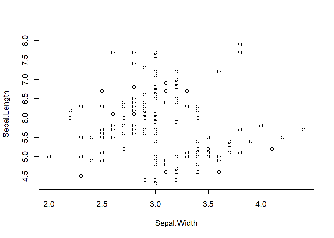

The data = argument informs the function about the dataset from which the variables (Sepal.Length and Sepal.Width) should be extracted.

Symbol

pch argument. Choose from 1 to 25 (google r plot pch for details)

plot(Sepal.Length ~ Sepal.Width, data = iris,
     pch = 19)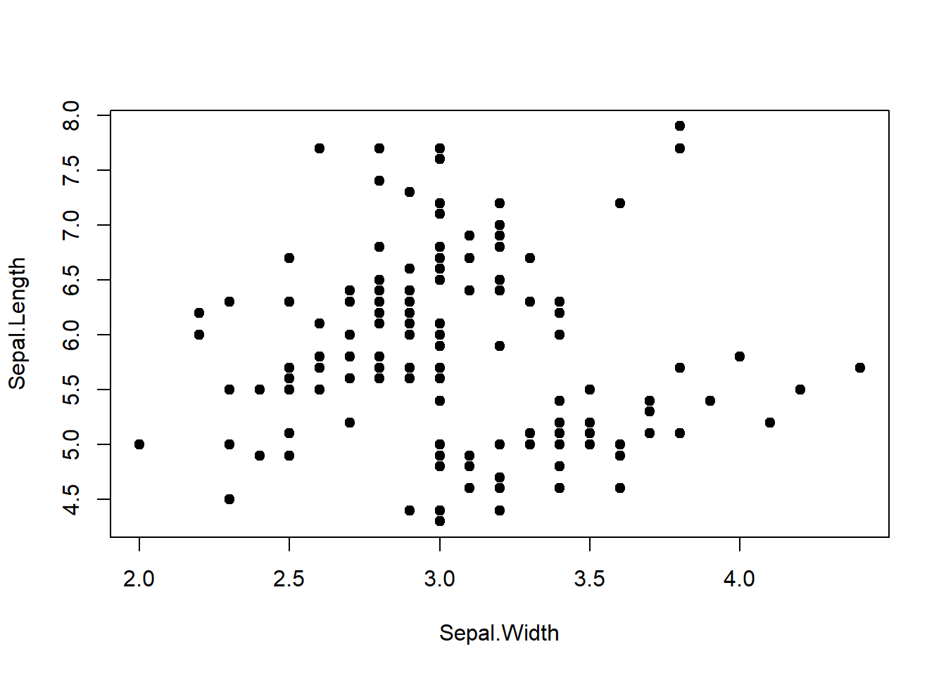

Symbol size

cex argument. cex = 1 is the default value. cex = 2 is as twice large as default value.

plot(Sepal.Length ~ Sepal.Width, data = iris,
     pch = 19, cex = 2)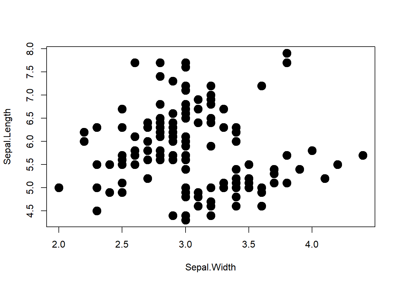

Symbol color (border)

col argument (quote "color name" when specifying). Google r color name for color options.

plot(Sepal.Length ~ Sepal.Width, data = iris,
     pch = 21, cex = 2, col = "gray")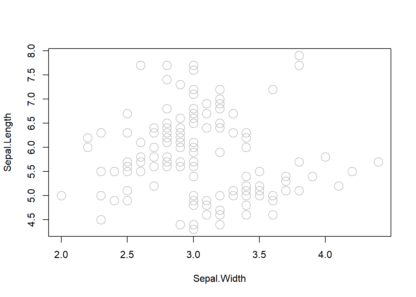

Symbol color (fill)

bg argument (quote "color name" when specifying). Available for a subset of symbol options (some symbols have pre-defined filled color).

plot(Sepal.Length ~ Sepal.Width, data = iris,
     pch = 21, cex = 2, bg = "lightgray")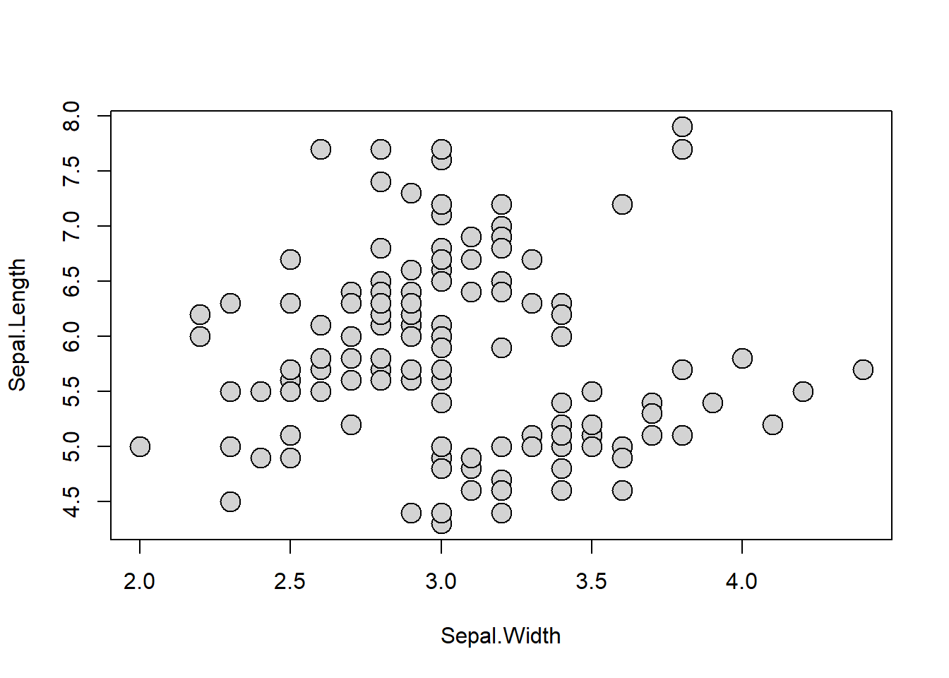

Label

ylab or xlab arguments. Provide "quoted text".

plot(Sepal.Length ~ Sepal.Width, data = iris,
     pch = 21, cex = 2, bg = "lightgray",
     xlab = "Sepal width (cm)", ylab = "Sepal length (cm)")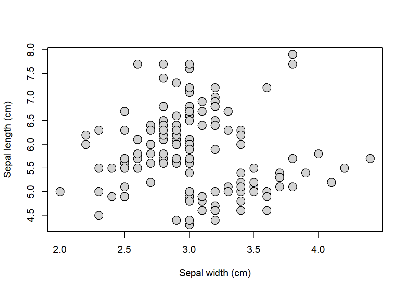

Axis

Delete axes with axes = F and re-draw with box() and axis() functions.

plot(Sepal.Length ~ Sepal.Width, data = iris,
     pch = 21, cex = 2, bg = "lightgray",
     xlab = "Sepal width (cm)", ylab = "Sepal length (cm)",
     axes = F)
box(bty = "l") # L-shaped border lines
axis(1) # 1: draw x-axis
axis(2, las = 2) # 2: draw y-axis, las = 2: make axis lables horizontal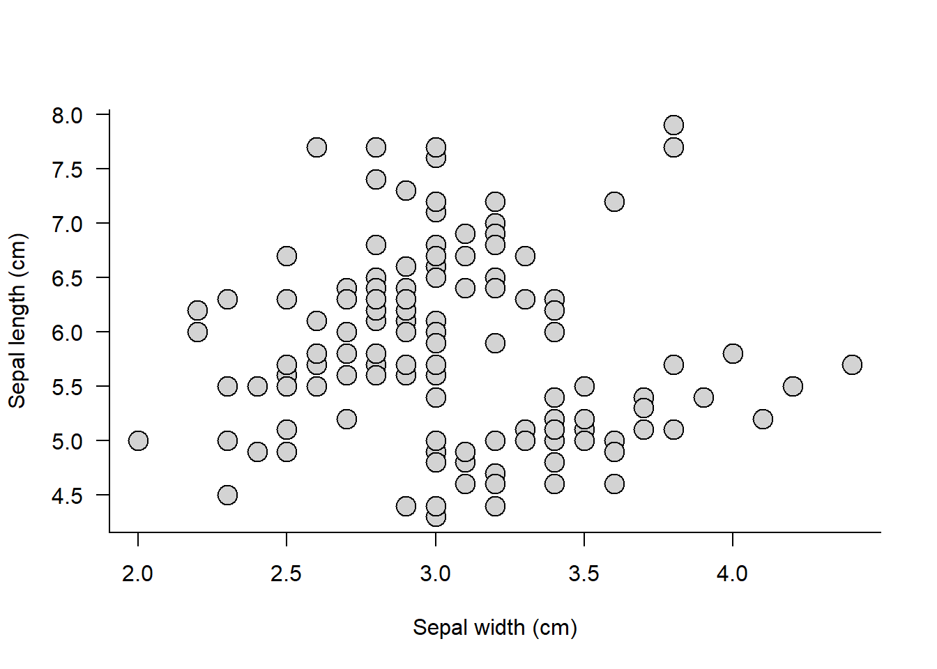

Boxplot

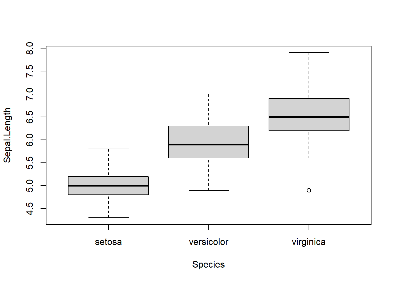
boxplot() is used when the x-axis is factor-type data (by default, plot() will produce a boxplot when x-axis is a factor variable). In the iris dataset, the column Species is a factor variable. Compare Sepal.Length among species using boxplot().

boxplot(Sepal.Length ~ Species, data = iris)

You can customize as in plot(), but slighlty different.

Box color

col argument.

boxplot(Sepal.Length ~ Species, data = iris,
        col = "lightgray")

Border color

border argument.

boxplot(Sepal.Length ~ Species, data = iris,
        col = "lightgray", border = "grey48")

Box width

boxwex argument.

boxplot(Sepal.Length ~ Species, data = iris,
        col = "lightgray", border = "grey48",
        boxwex = 0.4 )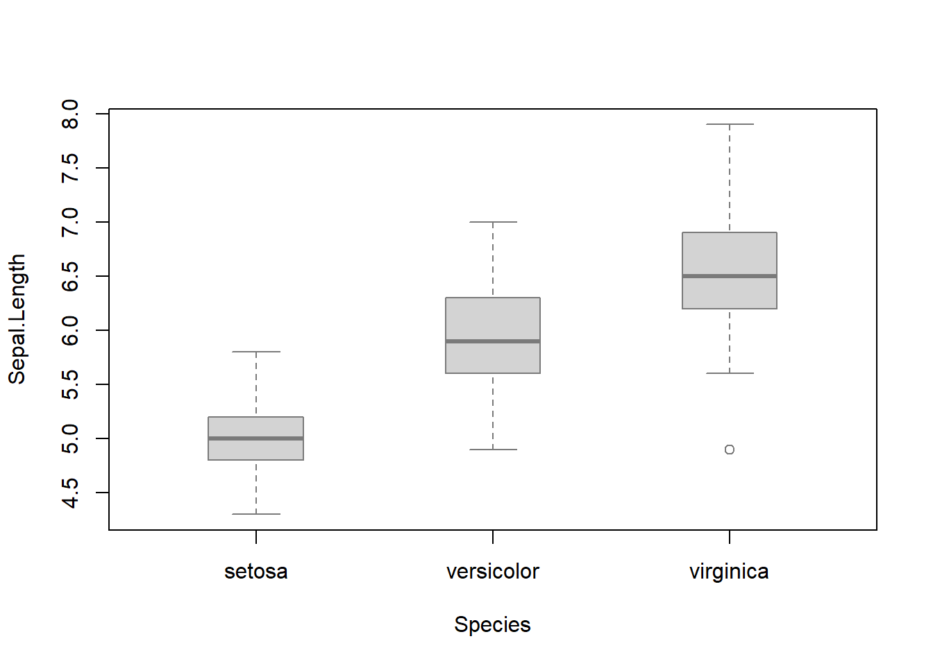

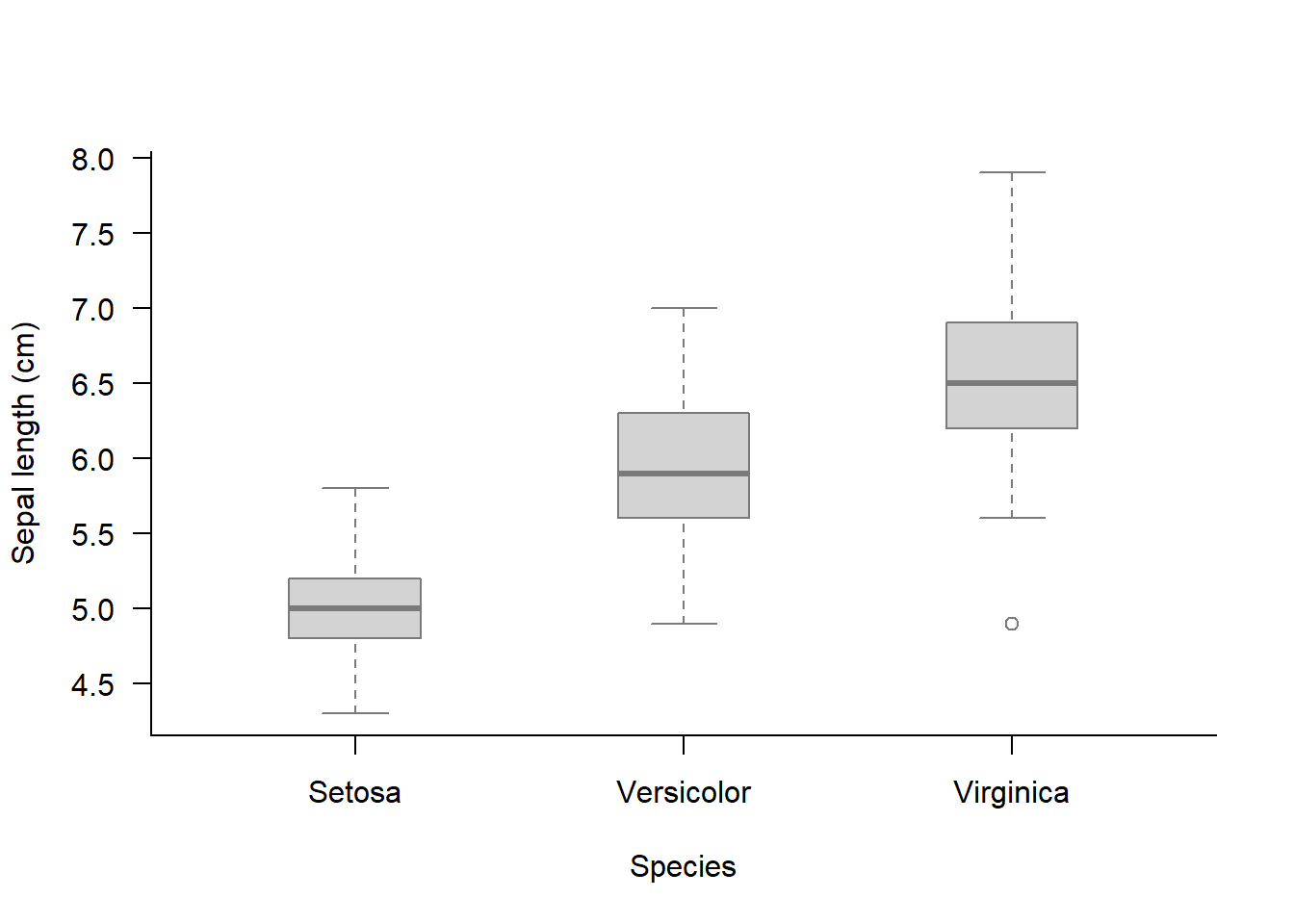
Axis

Delete axes with axes = F and re-draw with box() and axis() functions.

boxplot(Sepal.Length ~ Species, data = iris,
        col = "lightgray", border = "grey48",
        boxwex = 0.4, ylab = "Sepal length (cm)",
        axes = F)
box(bty = "l")
axis(1, at = c(1, 2, 3), labels = c("Setosa", "Versicolor", "Virginica") )
axis(2, las = 2)

Git & GitHub