12 Regression
Our previous examples focused on cases that involved a distinct group structure. However, it is not always the case that such a structure exists. Instead, we might examine the relationship between continuous variables. In this chapter, I will introduce a technique called linear regression.
Key words: intercept, slope (coefficient), least squares, residual, coefficient of determination (\(\mbox{R}^2\))
12.1 Explore Data Structure
For this exercise, we will use algae biomass data from streams. Download the data here and locate it in data_raw/.
## # A tibble: 50 × 4
##    biomass unit_biomass conductivity unit_cond
##      <dbl> <chr>               <dbl> <chr>
##  1   19.8  mg_per_m2            30.2 ms
##  2   24.4  mg_per_m2            40.4 ms
##  3   27.4  mg_per_m2            59.4 ms
##  4   48.2  mg_per_m2            91.3 ms
##  5   19.2  mg_per_m2            24.2 ms
##  6   57.0  mg_per_m2            90.4 ms
##  7   51.9  mg_per_m2            94.7 ms
##  8   40.8  mg_per_m2            67.8 ms
##  9   37.1  mg_per_m2            64.8 ms
## 10    3.55 mg_per_m2            10.9 ms
## # ℹ 40 more rows
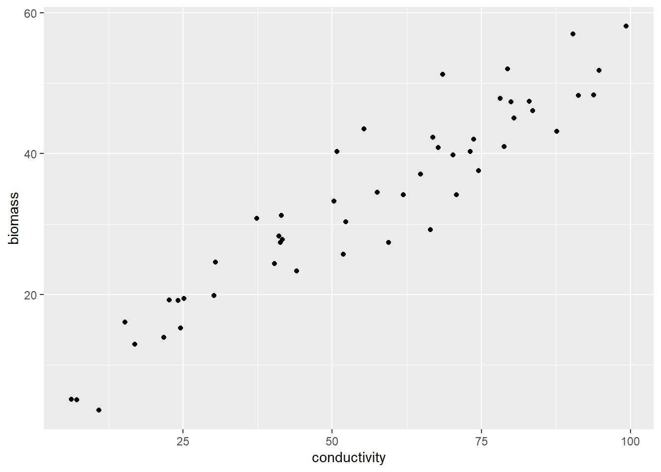
This dataset comprises data collected from 50 sampling sites. The variable biomass represents the standing biomass, indicating the dry mass of algae at the time of collection. On the other hand, conductivity serves as a proxy for water quality, with higher values usually indicating a higher nutrient content in the water. Let me now proceed to draw a scatter plot that will help visualize the relationship between these two variables.
df_algae %>%
  ggplot(aes(x = conductivity,
             y = biomass)) +
  geom_point()
Figure 12.1: The relationship between algae biomass and conductivity.
It seems that there is a noticeable positive correlation where increased conductivity results in higher algal biomass. Nevertheless, how can we accurately represent this relationship with a line?
12.2 Drawing the “fittest” line
12.2.1 Linear formula
The first step is to represent the relationship as a formula; let me ASSUME that the relationship can be described by the following linear formula:
\[ y_i = \alpha + \beta x_i \]
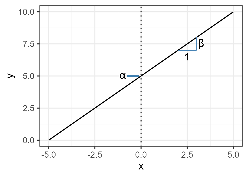
In this formula, the algal biomass, denoted as \(y_i\), at site \(i\), is expressed as a function of conductivity, represented by \(x_i\). The variable being explained (\(y_i\)) is referred to as a response (or dependent) variable, while the variable used to predict the response variable (\(x_i\)) is referred to as an explanatory (or independent) variable. However, there are two additional constants, namely \(\alpha\) and \(\beta\). \(\alpha\) is commonly known as the intercept, while \(\beta\) is referred to as the slope or coefficient. The intercept represents the value of \(y\) when \(x\) is equal to zero, while the slope indicates the change in \(y\) associated with a unit increase in \(x\) (refer to Figure 12.2).

Figure 12.2: Intercept and slope.
However, this formula, or “model,” is incomplete. We must add the error term \(\varepsilon_i\) (residual) to consider the uncertainty associated with the observation process.
\[ y_i = \alpha + \beta x_i + \varepsilon_i\\ \varepsilon_i \sim \text{Normal}(0, \sigma^2) \]
Notice that \(y_i\), \(x_i\), and \(\varepsilon_i\) have subscripts, while \(\alpha\) and \(\beta\) do not. This means that \(y_i\), \(x_i\), and \(\varepsilon_i\) vary by data point \(i\), and \(\alpha\) and \(\beta\) are constants. Although \(\alpha + \beta x_i\) cannot reproduce \(y_i\) perfectly, we “fill” the gaps with the error term \(\varepsilon_i\), which is assumed to follow a Normal distribution.
In R, finding the best \(\alpha\) and \(\beta\) – i.e., the parameters in this model – is very easy. Function lm() does everything for you. Let me apply this function to the example data set:
# lm() takes a formula as the first argument
# don't forget to supply your data
m <- lm(biomass ~ conductivity,
        data = df_algae)

summary(m)
##
## Call:
## lm(formula = biomass ~ conductivity, data = df_algae)
##
## Residuals:
## Min 1Q Median 3Q Max
## -9.5578 -2.8729 -0.7307 2.5479 11.4700
##
## Coefficients:
## Estimate Std. Error t value Pr(>|t|)
## (Intercept) 5.29647 1.57178 3.37 0.00149 **
## conductivity 0.50355 0.02568 19.61 < 2e-16 ***
## ---
## Signif. codes: 0 '***' 0.001 '**' 0.01 '*' 0.05 '.' 0.1 ' ' 1
##
## Residual standard error: 4.649 on 48 degrees of freedom
## Multiple R-squared: 0.889, Adjusted R-squared: 0.8867
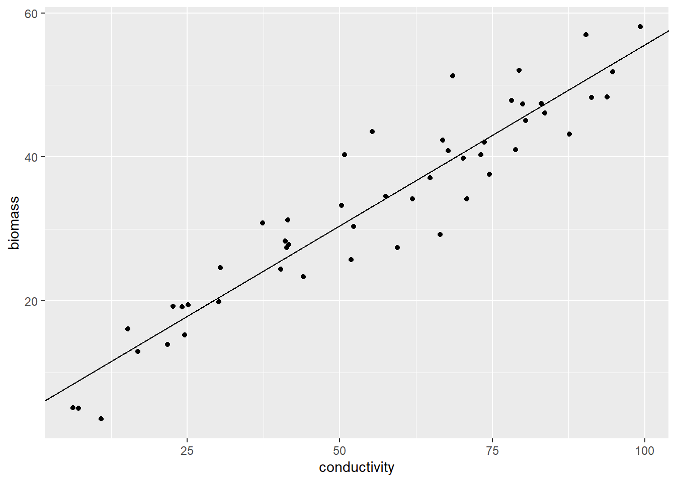
## F-statistic: 384.5 on 1 and 48 DF, p-value: < 2.2e-16In Coefficients:, it says (Intercept) is 5.3 and conductivity is 0.5. These values corresponds to \(\alpha\) and \(\beta\). Meanwhile, Residual standard error: indicates the SD of the error term \(\sigma\). Thus, substituting these values into the formula yields:
\[ y_i = 5.30 + 0.50 x_i + \varepsilon_i\\ \varepsilon_i \sim \text{Normal}(0, 4.6^2) \]
We can draw this “fittest” line on the figure:
# coef() extracts estimated coefficients
# e.g., coef(m)[1] is (Intercept)

alpha <- coef(m)[1]
beta <- coef(m)[2]

df_algae %>%
  ggplot(aes(x = conductivity,
             y = biomass)) +
  geom_point() +
  geom_abline(intercept = alpha,
              slope = beta) # draw the line
Figure 12.3: Drawing the fitted model prediction.
However, how did lm() find \(\alpha\) and \(\beta\)?
12.2.2 Minimizing the errors
Notice that the error term is the difference between \(y_i\) and \(\alpha + \beta x_i\):
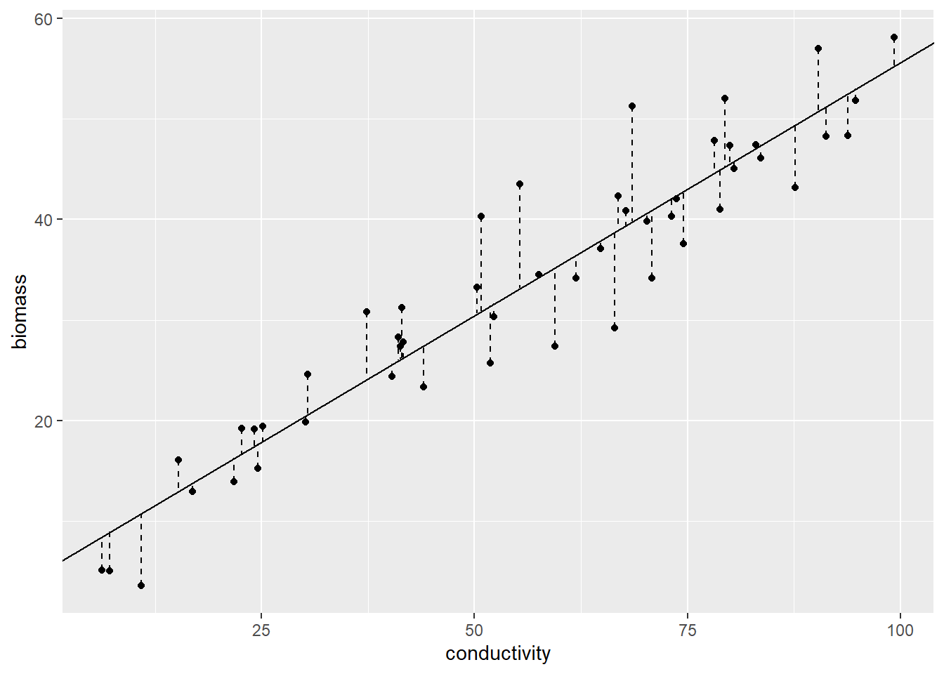
\[ \varepsilon_i = y_i - (\alpha + \beta x_i) \]In other words, this term represents the portion of the observation \(y_i\) that cannot be explained by the conductivity \(x_i\). Therefore, a logical approach would be to find values for \(\alpha\) and \(\beta\) that minimize this unexplained portion across all data points \(i\).
Least squares methods are a widely employed statistical approach to achieve this objective. These methods aim to minimize the sum of squared errors, denoted as \(\sum_i \varepsilon_i^2\), across all data points. As the deviation from the expected value of \(\alpha + \beta x_i\) increases, this quantity also increases. Consequently, determining parameter values (\(\alpha\) and \(\beta\)) that minimize this sum of squared errors yields the best-fitting formula (see Section 12.2.3 for further details).
12.2.3 Least Squares
Introducing a matrix representation is indeed a helpful way to explain the least square method. Here, I represent the vector of observed values \(y_i\) as \(Y\) (\(Y = \{y_1, y_2,...,y_n\}^T\)), the vector of parameters as \(\Theta\) (\(\Theta = \{\alpha, \beta\}^T\)), and the matrix composed of \(1\)s and \(x_i\) values as \(X\). The matrix \(X\) can be written as:
\[ X = \begin{pmatrix} 1 & x_1\\ 1 & x_2\\ 1 & x_3\\ \vdots & \vdots\\ 1 & x_n \end{pmatrix} \]
Using matrix notation, we can express the error vector \(\pmb{\varepsilon}\) as:
\[ \pmb{\varepsilon} = Y - X\Theta \]
The column of \(1\)s is required to represent the intercept; \(X\Theta\) reads:
\[ X\Theta = \begin{pmatrix} 1 & x_1\\ 1 & x_2\\ 1 & x_3\\ \vdots & \vdots\\ 1 & x_n \end{pmatrix} \begin{pmatrix} \alpha\\ \beta \end{pmatrix} = \begin{pmatrix} \alpha + \beta x_1\\ \alpha + \beta x_2\\ \alpha + \beta x_3\\ \vdots\\ \alpha + \beta x_n \end{pmatrix} \]
Minimizing the squared magnitude of \(\pmb{\varepsilon}\) (solve the partial derivative of \(||\pmb{\varepsilon}||^2\) about \(\Theta\)) leads to the solution (for detailed derivation, refer to Wikipedia):
\[ \hat{\Theta} = (X^TX)^{-1}X^{T}Y \]
Let me see if this reproduces the result of lm():
# create matrix X
v_x <- df_algae %>% pull(conductivity)
X <- cbind(1, v_x)

# create a vector of y
Y <- df_algae %>% pull(biomass)

# %*%: matrix multiplication
# t(): transpose a matrix
# solve(): computes the inverse matrix
theta <- solve(t(X) %*% X) %*% t(X) %*% Y
print(theta)
## [,1]
## 5.2964689
## v_x 0.5035548lm() output for a reference:
##  (Intercept) conductivity
##    5.2964689    0.5035548
12.2.4 Standard Errors and t-values
Ensuring the reliability of the estimated point estimates for \(\alpha\) and \(\beta\) is crucial. In the summary(m) output, two statistical quantities, namely the Std. Error and t-value, play a significant role in assessing the uncertainty associated with these estimates.
The standard error (Std. Error; “SE”) represents the estimated standard deviation of the parameter estimates (\(\hat{\theta}\) is either \(\hat{\alpha}\) or \(\hat{\beta}\)). A smaller value of the standard error indicates a higher degree of statistical reliability in the estimate. On the other hand, the t-value is a concept we have covered in Chapter 10. This value is defined as:
\[ t = \frac{\hat{\theta} - \theta_0}{\text{SE}(\hat{\theta})} \]
The t-statistic is akin to the t-test; however, in the context of regression analysis, we do not have another group to compare with (i.e., \(\theta_0\)). Typically, in regression analysis, we use zero as the reference (\(\theta_0 = 0\)). Therefore, higher t-values in lm() indicate a greater deviation from zero. Consequently, the Null Hypothesis in regression analysis is \(\beta = 0\). This hypothesis is sensible in our specific example since we are interested in quantifying the effect of conductivity. If \(\beta = 0\), it implies that conductivity has no effect on algal biomass. Since \(\theta_0 = 0\), the following code reproduces the reported t-values:
# extract coefficients
theta <- coef(m)

# extract standard errors
se <- sqrt(diag(vcov(m)))

# t-value
t_value <- theta / se
print(t_value)
## (Intercept) conductivity
## 3.369732 19.609446After defining the Null Hypothesis and t-values, we can compute the probability of observing the estimated parameters under the Null Hypothesis. Similar to the t-test, lm() utilizes a Student’s t-distribution for this purpose. However, the difference lies in how we estimate the degrees of freedom. In our case, we have 50 data points but need to subtract the number of parameters, which are \(\alpha\) and \(\beta\). Therefore, the degrees of freedom would be \(50 - 2 = 48\). This value is employed when calculating the p-value:
# for intercept
# (1 - pt(t_value[1], df = 48)) calculates pr(t > t_value[1])
# pt(-t_value[1], df = 48) calculates pr(t < -t_value[1])
p_alpha <- (1 - pt(t_value[1], df = 48)) + pt(-t_value[1], df = 48)

# for slope
p_beta <- (1 - pt(t_value[2], df = 48)) + pt(-t_value[2], df = 48)

print(p_alpha)
## (Intercept)
## 0.001492023
print(p_beta)## conductivity
## 7.377061e-2512.3 Unexplained Variation
12.3.1 Retrieve Errors
The function lm() provides estimates for \(\alpha\) and \(\beta\), but it does not directly provide the values of \(\varepsilon_i\). To gain a deeper understanding of the statistical model, it is necessary to examine the residuals \(\varepsilon_i\). By using the resid() function, you can obtain the values of \(\varepsilon_i\). This allows you to explore and extract insights from the developed statistical model.
##          1          2          3          4          5          6
## -0.6838937 -1.2149034 -7.8576927 -3.0109473  1.7076481  6.1773586
Each element retains the order of data point in the original data frame, so eps[1] (\(\varepsilon_1\)) should be identical to \(y_1 - (\alpha + \beta x_1)\). Let me confirm:
# pull vector data
v_x <- df_algae %>% pull(conductivity)
v_y <- df_algae %>% pull(biomass)

# theta[1] = alpha
# theta[2] = beta
error <- v_y - (theta[1] + theta[2] * v_x)

# cbind() combines vectors column-wise
# head() retrieves the first 6 rows
head(cbind(eps, error))
## eps error
## 1 -0.6838937 -0.6838937
## 2 -1.2149034 -1.2149034
## 3 -7.8576927 -7.8576927
## 4 -3.0109473 -3.0109473
## 5 1.7076481 1.7076481
## 6 6.1773586 6.1773586To ensure that the two columns are indeed identical, a visual check may be prone to overlooking small differences. To perform a more precise comparison, you can use the all() function to check if the data aligns (here, evaluated at the five decimal points using round()). By comparing the two columns in this manner, you can confirm whether they are identical or not.
# round values at 5 decimal
eps <- round(eps, 5)
error <- round(error, 5)

# eps == error return "TRUE" or "FALSE"
# all() returns TRUE if all elements meet eps == error
all(eps == error)
## [1] TRUE12.3.2 Visualize Errors
To visualize the errors or residuals, which represent the distance from the best-fitted line to each data point, you can make use of the geom_segment() function:
# add error column
df_algae <- df_algae %>%
  mutate(eps = eps)

df_algae %>%
  ggplot(aes(x = conductivity,
             y = biomass)) +
  geom_point() +
  geom_abline(intercept = alpha,
              slope = beta) +
  geom_segment(aes(x = conductivity, # start-coord x
                   xend = conductivity, # end-coord x
                   y = biomass, # start-coord y
                   yend = biomass - eps), # end-coord y
               linetype = "dashed")
Figure 12.4: Vertical segments indicate errors.
12.3.3 Coefficient of Determination
One crucial motivation for developing a regression model, or any statistical model, is to assess the extent to which the explanatory variable (\(x_i\)) explains the variation in the response variable (\(y_i\)). By fitting a regression model, we can quantify the amount of variability in the response variable that can be attributed to the explanatory variable. This assessment provides valuable insights into the strength and significance of the relationship between the variables under consideration.
The coefficient of determination, denoted as R², is a statistical measure that assesses the proportion of the variance in the response variable that can be explained by the explanatory variable(s) in a regression model. It provides an indication of how well the regression model fits the observed data. The formula for R² is:
\[ \text{R}^2 = 1 - \frac{SS}{SS_0} \]
where \(SS\) is the summed squares of residuals (\(\sum_i \varepsilon_i^2\)), and \(SS_0\) is the summed squares of the response variable (\(SS_0 = \sum_i(y_i - \hat{\mu}_y)^2\)). The term \(\frac{SS}{SS_0}\) represents the proportion of variability “unexplained” – therefore, \(1 - \frac{SS}{SS_0}\) gives the proportion of variability “explained.” R² is a value between 0 and 1. An R² value of 0 indicates that the explanatory variable(s) cannot explain any of the variability in the response variable, while an R² value of 1 indicates that the explanatory variable(s) can fully explain the variability in the response variable.
While R2 is provided as a default output of lm(), let’s confirm if the above equation reproduces the reported value:
# residual variance
ss <- sum(resid(m)^2)

# null variance
ss_0 <- sum((v_y - mean(v_y))^2)

# coefficient of determination
r2 <- 1 - ss / ss_0

print(r2)
## [1] 0.8890251Compare it with lm() output:
summary(m)##
## Call:
## lm(formula = biomass ~ conductivity, data = df_algae)
##
## Residuals:
## Min 1Q Median 3Q Max
## -9.5578 -2.8729 -0.7307 2.5479 11.4700
##
## Coefficients:
## Estimate Std. Error t value Pr(>|t|)
## (Intercept) 5.29647 1.57178 3.37 0.00149 **
## conductivity 0.50355 0.02568 19.61 < 2e-16 ***
## ---
## Signif. codes: 0 '***' 0.001 '**' 0.01 '*' 0.05 '.' 0.1 ' ' 1
##
## Residual standard error: 4.649 on 48 degrees of freedom
## Multiple R-squared: 0.889, Adjusted R-squared: 0.8867
## F-statistic: 384.5 on 1 and 48 DF, p-value: < 2.2e-16Multiple R-squared: corresponds to the calculated coefficient of determination.
12.4 Laboratory
12.4.1 Develop regression models
R provides a built-in data set called iris. The iris data contain data points from three different species (Species column). Split this data set by species (create three separate data frames) and perform regression for each species separately to analyze the relationship between Sepal.Width (response variable) and Petal.Width (explanatory variable).
head(iris)## Sepal.Length Sepal.Width Petal.Length Petal.Width Species
## 1 5.1 3.5 1.4 0.2 setosa
## 2 4.9 3.0 1.4 0.2 setosa
## 3 4.7 3.2 1.3 0.2 setosa
## 4 4.6 3.1 1.5 0.2 setosa
## 5 5.0 3.6 1.4 0.2 setosa
## 6 5.4 3.9 1.7 0.4 setosa12.4.2 Multiple explanatory variables
Regression analysis can involve multiple explanatory variables. To explore this, consider utilizing Petal.Length as an additional explanatory variable for each species. Then, investigate (1) the variations in estimates of regression coefficients and (2) the differences in the coefficients of determination compared to the model with only a single explanatory variable.