10 Two-Group Comparison
Data consists of “samples” extracted from the population of interest, but it’s important to acknowledge that these samples are not flawless replicas of the entire population. Given this imperfect information, how can we effectively investigate and discern the distinction between two populations? In this Chapter, I will introduce one of the most basic statistical tests – “t-test.” The t-test takes the following steps:
- Define a test statistic to signify the difference between groups (t-statistic).
- Define a probability distribution of t-statistic under the null hypothesis, i.e., a scenario that we assume no difference between groups.
- Estimate the probability of yielding greater or less than the observed test statistic under the null hypothesis.
Key words: t-statistic, null hypothesis, alternative hypothesis, p-value
10.1 Explore Data Structure
Suppose that we study fish populations of the same species in two lakes (Lake a and b). These lakes are in stark contrast of productivity (Lake b looks more productive), and our interest is the difference in mean body size between the two lakes. We obtained \(50\) data points of fish length from each lake (download here). Save under data_raw/ and use read_csv() to read data:
library(tidyverse) # call add-in packages everytime you open new R session
df_fl <- read_csv("data_raw/data_fish_length.csv")
print(df_fl)
## # A tibble: 100 × 3
## lake length unit
## <chr> <dbl> <chr>
## 1 a 10.8 cm
## 2 a 13.6 cm
## 3 a 10.1 cm
## 4 a 18.6 cm
## 5 a 14.2 cm
## 6 a 10.1 cm
## 7 a 14.7 cm
## 8 a 15.6 cm
## 9 a 15 cm
## 10 a 11.9 cm
## # ℹ 90 more rowsIn this data frame, fish length data from lake a and b are recorded. Confirm this with unique() or distinct() function:
# unique returns unique values as a vector
unique(df_fl$lake)
## [1] "a" "b"
# distinct returns unique values as a tibble
distinct(df_fl, lake)
## # A tibble: 2 × 1
## lake
## <chr>
## 1 a
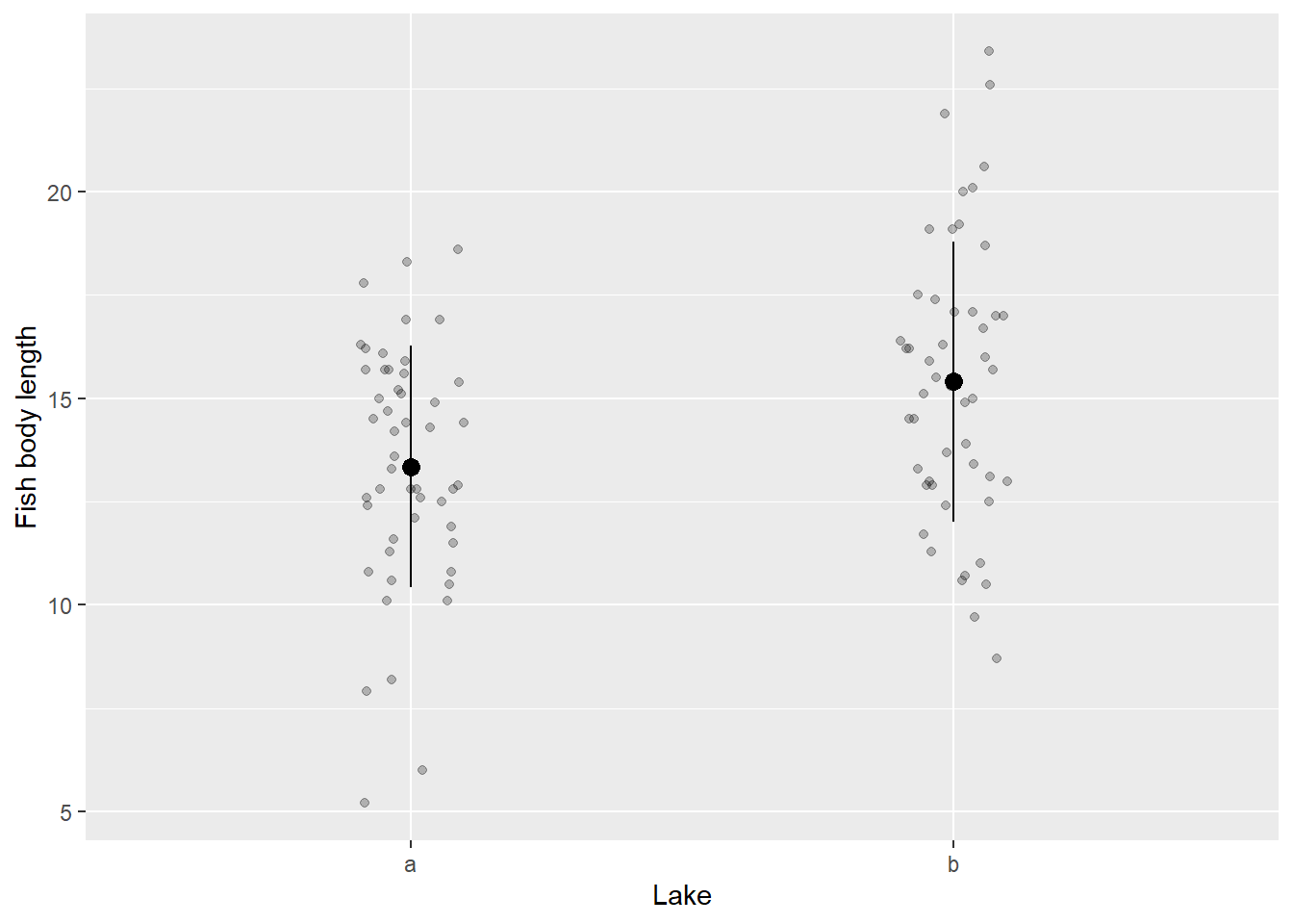
## 2 bVisualization provides a powerful tool for summarizing data effectively. By plotting individual data points overlaid with mean values and error bars, we can observe the distribution and patterns within the data, allowing us to identify trends, variations, and potential outliers:
# group mean and sd
df_fl_mu <- df_fl %>%
  group_by(lake) %>% # group operation
  summarize(mu_l = mean(length), # summarize by mean()
            sd_l = sd(length)) # summarize with sd()

# plot
# geom_jitter() plot data points with scatter
# geom_segment() draw lines
# geom_point() draw points
df_fl %>%
  ggplot(aes(x = lake,
             y = length)) +
  geom_jitter(width = 0.1, # scatter width
              height = 0, # scatter height (no scatter with zero)
              alpha = 0.25) + # transparency of data points
  geom_segment(data = df_fl_mu, # switch data frame
               aes(x = lake,
                   xend = lake,
                   y = mu_l - sd_l,
                   yend = mu_l + sd_l)) +
  geom_point(data = df_fl_mu, # switch data frame
             aes(x = lake,
                 y = mu_l),
             size = 3) +
  labs(x = "Lake", # x label
       y = "Fish body length") # y label
Figure 10.1: Example of mean and SD plot
Hmm, it is possible that there is a noticeable disparity in body size between Lake a and Lake b. However, how can we ascertain and provide evidence for this claim?
10.2 t-test in R
For this simple data set, we can use t-test. R provides t.test() function to perform this analysis:
x <- df_fl %>%
  filter(lake == "a") %>%  # subset lake a
  pull(length)

y <- df_fl %>%
  filter(lake == "b") %>% # subset lake b
  pull(length)

t.test(x, y, var.equal = TRUE)
##
## Two Sample t-test
##
## data: x and y
## t = -3.2473, df = 98, p-value = 0.001596
## alternative hypothesis: true difference in means is not equal to 0
## 95 percent confidence interval:
## -3.3124399 -0.7995601
## sample estimates:
## mean of x mean of y
## 13.350 15.406The reported t-statistic t = -3.2473, the p-value p-value = 0.001596, and the degrees of freedom all agreed (df = 98) – however, what do these values mean? How are we supposed to interpret t = -3.2473 and p-value = 0.001596?
10.3 Test Statistic
10.3.1 t-statistic
The starting point is to define what we want to look at. Since our focus is on examining the difference in means, it is logical to estimate the disparity between the sample means in each lake. Let me denote the sample means as \(\hat{\mu}_a\) and \(\hat{\mu}_b\) for Lake a and Lake b, respectively. We can estimate the difference between the means using the following approach:
# take another look at df_fl_mu
print(df_fl_mu)
## # A tibble: 2 × 3
## lake mu_l sd_l
## <chr> <dbl> <dbl>
## 1 a 13.4 2.92
## 2 b 15.4 3.39## [1] 13.35
# lake b
print(v_mu[2])
## [1] 15.406
# difference
v_mu[1] - v_mu[2]
## [1] -2.056The average fish body size in Lake b is approximately 2 cm larger than that in Lake a. However, it is crucial to recognize that we are still lacking vital information, specifically, the uncertainty associated with this difference. As discussed in Chapter 8, we must acknowledge that sample means are not flawless representations of the entire population.
Fortunately, we can utilize sample variances to address such uncertainties. The t-statistic is a common indicator of the difference of means that takes into consideration the uncertainty associated with sample means.
\[ t = \frac{\hat{\mu_a} - \hat{\mu_b}}{\sqrt{\hat{\sigma}^2_p \left(\frac{1}{N_a} + \frac{1}{N_b}\right)}} \]
where \(N_a\) and \(N_b\) are sample sizes in Lake a and b (i.e., \(N_a = N_b = 50\) in this specific example), and \(\hat{\sigma}^2_p\) is the weighted mean of sample variances:
\[ \hat{\sigma}^2_p = \frac{N_a-1}{N_a + N_b - 2}\hat{\sigma}^2_a + \frac{N_b-1}{N_a + N_b - 2}\hat{\sigma}^2_b \]
We can calculate this value in R manually:
# group mean, variance, and sample size
df_t <- df_fl %>%
  group_by(lake) %>% # group operation
  summarize(mu_l = mean(length), # summarize by mean()
            var_l = var(length), # summarize with sd()
            n = n()) # count number of rows per group

print(df_t)
## # A tibble: 2 × 4
## lake mu_l var_l n
## <chr> <dbl> <dbl> <int>
## 1 a 13.4 8.52 50
## 2 b 15.4 11.5 50
# pull values as a vector
v_mu <- pull(df_t, mu_l)
v_var <- pull(df_t, var_l)
v_n <- pull(df_t, n)

var_p <- ((v_n[1] - 1)/(sum(v_n) - 2)) * v_var[1] +
  ((v_n[2] - 1)/(sum(v_n) - 2)) * v_var[2]

t_value <- (v_mu[1] - v_mu[2]) / sqrt(var_p * ((1 / v_n[1]) + (1 / v_n[2])))

print(t_value)
## [1] -3.247322The difference in sample means were -2.06; therefore, t-statistic further emphasizes the distinction between the study lakes. This occurrence can be attributed to the t-statistic formula.
In the denominator, we observe the inclusion of \(\hat{\sigma}^2_p\) (estimated pooled variance), as well as the inverses of sample sizes \(N_a\) and \(N_b\). Consequently, as \(\hat{\sigma}^2_p\) decreases and/or the sample sizes increase, the t-statistic increases. This is a reasonable outcome since a decrease in variance and/or an increase in sample size enhance the certainty of the mean difference.
10.3.2 Null Hypothesis
The observed t-statistic serves a dual purpose in accounting for both the disparity of means and the accompanying uncertainty. However, the significance of this t-statistic remains unclear.
To address this, the concept of the Null Hypothesis is utilized to substantiate the observed t-statistic. The Null Hypothesis, no difference between groups or \(\mu_a = \mu_b\), allows us to draw the probability distribution of the test-statistic. Once we know the probability distribution, we can estimate the probability of observing the given t-statistic by random chance if there were no difference in mean body size between the lakes.
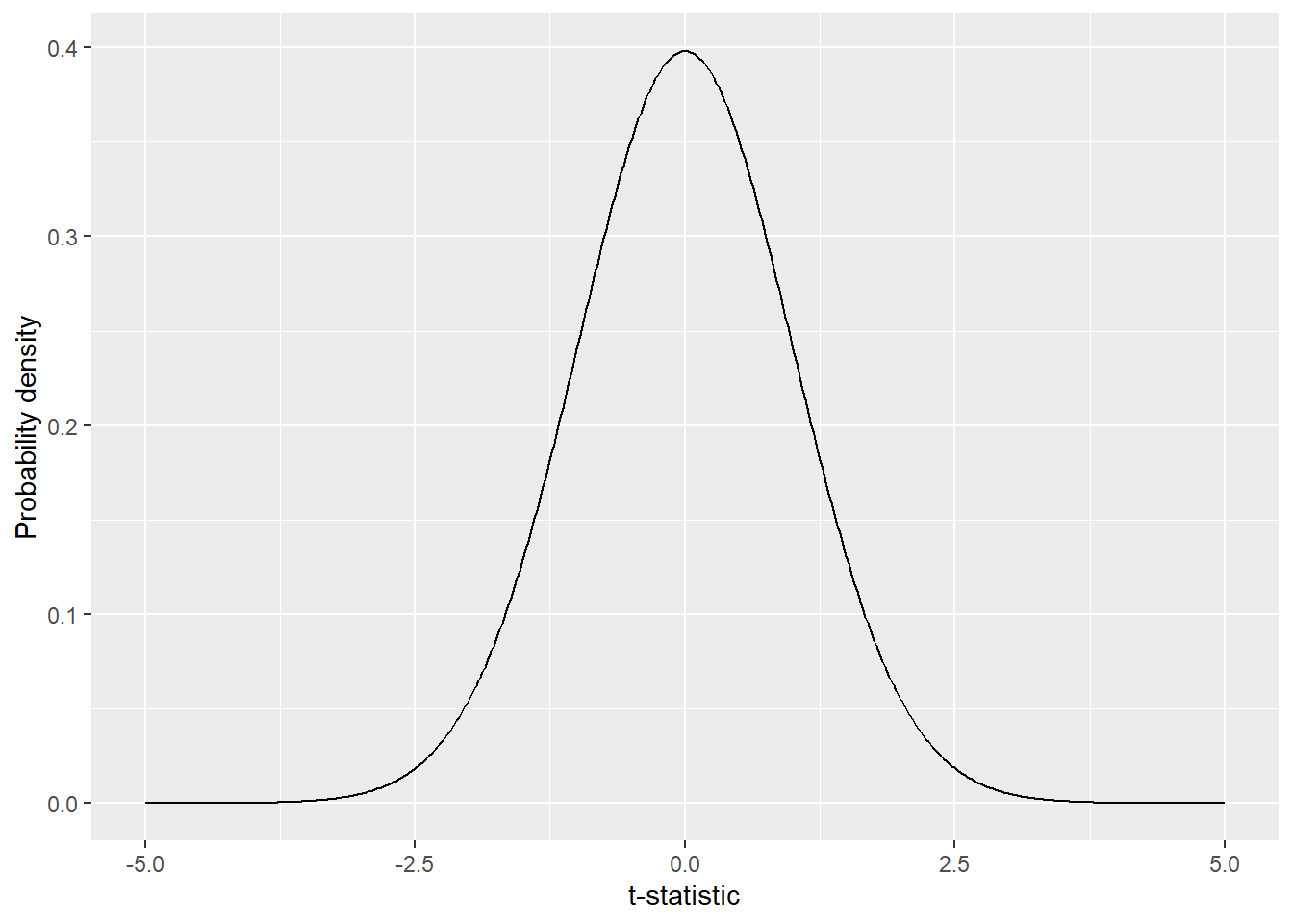
Let’s begin by assuming that there is no difference in the mean body size of fish populations between the lakes, meaning the true difference in means is zero (\(\mu_a - \mu_b = 0\); without hats in this formula!). Under this assumption, we can define the probability distribution of t-statistics, which represents how t-statistics are distributed across a range of possible values.
This probability distribution is known as the Student’s t-distribution and is characterized by three parameters: the mean, the variance, and the degrees of freedom (d.f.). Considering that we are evaluating the difference in body size as the test statistic, the mean (of the difference) is assumed to be zero. The variance is estimated using \(\hat{\sigma}^2_p\), and the degrees of freedom are determined by \(N_a + N_b - 2\) (where d.f. can be considered as a measure related to the sample size3).
R has a function to draw the Student’s t-distribution; let’s try that out:
# produce 500 values from -5 to 5 with equal interval
x <- seq(-5, 5, length = 500)

# probability density of t-statistics with df = sum(v_n) - 2
y <- dt(x, df = sum(v_n) - 2)

# draw figure
tibble(x, y) %>%
  ggplot(aes(x = x,
             y = y)) +
  geom_line() +
  labs(y = "Probability density",
       x = "t-statistic")
Figure 10.2: Distribution of t-statistics under null hypothesis. The probability density in a distribution determines the likelihood of observing a particular t-statistic. Higher probability density indicates a greater likelihood of the t-statistic occurring.
The probability density in a distribution (Figure 10.2) determines the likelihood of observing a particular t-statistic. Higher probability density indicates a greater likelihood of the t-statistic occurring. Compare the observed t-statistic against this null distribution:
# draw entire range
tibble(x, y) %>%
  ggplot(aes(x = x,
             y = y)) +
  geom_line() +
  geom_vline(xintercept = t_value,
             color = "salmon") + # t_value is the observed t_value
  geom_vline(xintercept = abs(t_value),
             color = "salmon") + # t_value is the observed t_value
  labs(y = "Probability density",
x = "t-statistic") 
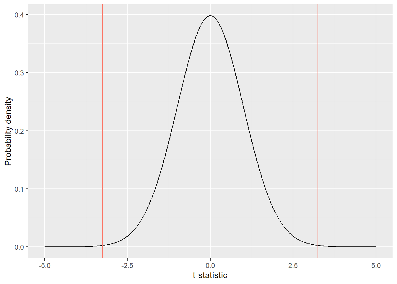
Figure 10.3: Observed t-statistic in comparison to the null distrubution
In a probability distribution, the area under the curve corresponds to the probability. Notably, the area under the curve that falls below or above the observed t-statistic (indicated by vertical red lines) is very small (Figure 10.3), meaning that the observed difference in body size is very unlikely to occur under the null hypothesis (no difference in true means).
The function pt() allows us to calculate the area under the curve:
# calculate area under the curve from -infinity to t_value
pr_below <- pt(q = t_value, df = sum(v_n) - 2)

# calculate area under the curve from abs(t_value) to infinity
pr_above <- 1 - pt(q = abs(t_value), df = sum(v_n) - 2)
The p-value, i.e., the probability of observing t-statistics less than ( pr_below) or greater than (pr_above) the observed t-statistic under the null hypothesis, can be estimated as the sum of pr_below and pr_above.
# p_value
p_value <- pr_below + pr_above
print(p_value)
## [1] 0.00159552910.3.3 Interpretation
The above exercise is called t-test – perhaps, the most well-known hypothesis testing. To explain the interpretation of the results, let me use the following notations. \(t_{obs}\), the observed t-statistic; \(t_0\), possible t-statistics under the null hypothesis; \(\Pr(\cdot)\), the probability of “\(\cdot\)” occurs – for example, \(\Pr(x > 2)\) means that the probability of \(x\) exceeding \(2\).
We first calculated the observed t-statistic \(t_{obs}\) using the data of fish body size, which was -3.25. Then, we calculated p-value, i.e., \(\Pr(t_0 < t_{obs}) + \Pr(t_0 > t_{obs})\) under the null hypothesis of \(\mu_a = \mu_b\). We found p-value was very low, meaning that the observed t-statistic is very unlikely to occur if \(\mu_a = \mu_b\) is the truth. Therefore, it is logical to conclude that the Alternative Hypothesis \(\mu_a \ne \mu_b\) is very likely.
The same logic is used in many statistical analyses – define the null hypothesis, and estimate the probability of observing a given value under the null hypothesis. It is tricky, but I find this genius: we can substantiate the observation(s) objectively that are otherwise a subjective claim!
However, it is crucial to recognize that, even if we found the observed t-statistic that results in very high p-value (i.e., very common under the null hypothesis), finding such a result does NOT support the null hypothesis – we just can’t reject it.
10.4 t-test with unequal variance
The above example assumes the relative similarity of variance between groups, which could be an unrealistic assumption. Luckily, there is a variant of t-test “Welch’s t-test,” in which we assume unequal variance between groups. The implementation is easy – set var.equal = FALSE in t.test():
t.test(x, y, var.equal = FALSE)##
## Welch Two Sample t-test
##
## data: x and y
## t = -0.7699, df = 501.15, p-value = 0.4417
## alternative hypothesis: true difference in means is not equal to 0
## 95 percent confidence interval:
## -0.3544786 0.1548791
## sample estimates:
## mean of x mean of y
## -2.029679e-16 9.979976e-02In Welch’s t-test, t-statistics are defined differently to account for unequal variance between groups4:
\[ t = \frac{\hat{\mu_a} - \hat{\mu_b}}{\sqrt{\left(\frac{\hat{\sigma}^2_a}{N_a} + \frac{\hat{\sigma}^2_b}{N_b}\right)}} \]
This t-statistic is known to follow the Student’s t-distribution with the degrees of freedom:
\[ d.f. = \frac{(\frac{\hat{\sigma}^2_a}{N_a} + \frac{\hat{\sigma}^2_b}{N_b})^2}{\frac{(\hat{\sigma}^2_a / N_a)^2}{N_a - 1} + \frac{(\hat{\sigma}^2_b/N_b)^2}{N_b-1}} \]
Therefore, the reported values of t-statistic and d.f. are different from what we estimated. The Welch’s t-test covers the cases for equal variances; therefore, by default, we use the Welch’s test.
10.5 Laboratory
10.5.1 Influence of Sample Size
Create the following vectors with rnorm():
-
xswith mean \(10\), SD \(5\), and sample size \(10\) -
yswith mean \(12\), SD \(5\), and sample size \(10\) -
xlwith mean \(10\), SD \(5\), and sample size \(100\) -
ylwith mean \(12\), SD \(5\), and sample size \(100\)
Perform Welch’s t-test for xs vs. ys, and xl vs. yl and compare p-values. Set var.equal = TRUE in t.test().
10.5.2 Difference and Uncertainty
We have four vectors - a1 and a2 & b1 and b2.
a1 <- c(13.9, 14.9 ,13.4, 14.3, 11.8, 13.9, 14.5, 15.1, 13.3, 13.9)
a2 <- c(17.4, 17.3, 20.1, 17.2, 18.4, 19.6, 16.8, 18.7, 17.8, 18.9)

b1 <- c(10.9, 20.3, 9.6, 8.3, 14.5, 12.3, 14.5, 16.7, 9.3, 22.0)
b2 <- c(26.9, 12.9, 11.1, 16.7, 20.0, 20.9, 16.6, 15.4, 16.2, 16.2)
Perform the following analysis:
Estimate sample means and SDs for each vector. To do so, create a
tibble()object withgroup(consist of charactersa1,a2,b1,b2) andvaluecolumns (consist of values above). Then usegroup_by()andsummarize()functions to estimate means and SDs for eachgroup.Create a figure similar to Figure 10.1 using data from
a1anda2.Perform Welch’s t-test for each pair and compare results.