13 Linear Model

We have extensively covered three important statistical analyses: the t-test, ANOVA, and regression analysis. While these methods may seem distinct, they all fall under the umbrella of the Linear Model framework⁵.

The Linear Model encompasses models that depict the connection between a response variable and one or more explanatory variables. It assumes that the error term follows a normal distribution. In this chapter, I will elucidate this framework and illustrate its relationship to the t-test, ANOVA, and regression analysis.

Key words: level of measurement, dummy variable

13.1 The Frame

The apparent distinctiveness between the t-test, ANOVA, and regression analysis arises because they are applied to different types of data:

• t-test: comparing differences between two groups.
• ANOVA: examining differences among more than two groups.
• Regression: exploring the relationship between a response variable and one or more explanatory variables.

Despite these differences, these analyses can be unified under a single formula. As discussed in the regression formula in Chapter 12, we have:

\[ \begin{aligned} y_i &= \alpha + \beta_1 x_{1,i} + \varepsilon_i\\ \varepsilon_i &\sim \text{Normal}(0, \sigma^2) \end{aligned} \]

where \(y_i\) represents the response variable (such as fish body length or plant height), \(x_{1,i}\) denotes the continuous explanatory variable, \(\alpha\) represents the intercept, and \(\beta_1\) corresponds to the slope. The equivalent model can be expressed differently as follows:

\[ \begin{aligned} y_i &\sim \text{Normal}(\mu_i, \sigma^2)\\ \mu_i &= \alpha + \beta_1 x_{1,i} \end{aligned} \]

This structure provides insight into the relationship between the t-test, ANOVA, and regression analysis. The fundamental purpose of regression analysis is to model how the mean \(\mu_i\) changes with increasing or decreasing values of \(x_{1,i}\). Thus, the t-test, ANOVA, and regression all analyze the mean – the expected value of a Normal distribution. The primary distinction between the t-test, ANOVA, and regression lies in the nature of the explanatory variable, which can be either continuous or categorical (group).

13.1.1 Two-Group Case

To establish a connection among these approaches, one can employ “dummy indicator” variables to represent group variables. In the case of the t-test, where a categorical variable consists of two groups, typically denoted as a and b (although they can be represented by numbers as well), one can convert these categories into numerical values. For instance, assigning a to 0 and b to 1 enables the following conversion:

\[ \pmb{x'}_2 = \begin{pmatrix} a\\ a\\ b\\ \vdots\\ b\end{pmatrix} \rightarrow \pmb{x}_2 = \begin{pmatrix} 0\\ 0\\ 1\\ \vdots\\ 1 \end{pmatrix} \]

The model can be written as:

\[ \begin{aligned} y_i &\sim \text{Normal}(\mu_i, \sigma^2)\\ \mu_i &= \alpha + \beta_2 x_{2,i} \end{aligned} \]

When incorporating this variable into the model, some interesting outcomes arise. Since \(x_{2,i} = 0\) when an observation belongs to group a, the mean of group a (\(\mu_i = \mu_a\)) is determined as \(\mu_a = \alpha + \beta \times 0 = \alpha\). Consequently, the intercept represents the mean value of the first group. On the other hand, if an observation is from group b, the mean of group b (\(\mu_i = \mu_b\)) is given by \(\mu_b = \alpha + \beta \times 1 = \alpha + \beta\). It’s important to recall that \(\mu_a = \alpha\). By substituting \(\alpha\) with \(\mu_a\), the equation \(\beta = \mu_b - \mu_a\) is obtained, indicating that the slope represents the difference between the means of the two groups – the key statistic in the t-test.

Let me confirm this using the dataset in Chapter 10 (fish body length in two lakes):

library(tidyverse)
df_fl <- read_csv("data_raw/data_fish_length.csv")
print(df_fl)

## # A tibble: 100 × 3
##    lake  length unit 
##    <chr>  <dbl> <chr>
##  1 a       10.8 cm   
##  2 a       13.6 cm   
##  3 a       10.1 cm   
##  4 a       18.6 cm   
##  5 a       14.2 cm   
##  6 a       10.1 cm   
##  7 a       14.7 cm   
##  8 a       15.6 cm   
##  9 a       15   cm   
## 10 a       11.9 cm   
## # ℹ 90 more rows

In the lm() function, when you provide a “categorical” variable in character or factor form, it is automatically converted to a binary (0/1) variable internally. This means that you can include this variable in the formula as if you were conducting a standard regression analysis. The lm() function takes care of this conversion process, allowing you to seamlessly incorporate categorical variables into the lm() function.

# group means
v_mu <- df_fl %>% 
  group_by(lake) %>% 
  summarize(mu = mean(length)) %>% 
  pull(mu)

# mu_a: should be identical to intercept
v_mu[1]

## [1] 13.35

# mu_b - mu_a: should be identical to slope
v_mu[2] - v_mu[1]

## [1] 2.056

# in lm(), letters are automatically converted to 0/1 binary variable.
# alphabetically ordered (in this case, a = 0, b = 1)
m <- lm(length ~ lake,
        data = df_fl)

summary(m)

## 
## Call:
## lm(formula = length ~ lake, data = df_fl)
## 
## Residuals:
##    Min     1Q Median     3Q    Max 
## -8.150 -2.156  0.022  2.008  7.994 
## 
## Coefficients:
##             Estimate Std. Error t value Pr(>|t|)    
## (Intercept)  13.3500     0.4477  29.819   <2e-16 ***
## lakeb         2.0560     0.6331   3.247   0.0016 ** 
## ---
## Signif. codes:  0 '***' 0.001 '**' 0.01 '*' 0.05 '.' 0.1 ' ' 1
## 
## Residual standard error: 3.166 on 98 degrees of freedom
## Multiple R-squared:  0.09715,    Adjusted R-squared:  0.08794 
## F-statistic: 10.55 on 1 and 98 DF,  p-value: 0.001596

The estimated coefficient of Lake b (lakeb) is identical to the difference between group means. We can compare other statistics (t value and Pr(>|t|) with the output from t.test() as well:

lake_a <- df_fl %>% 
  filter(lake == "a") %>% 
  pull(length)

lake_b <- df_fl %>% 
  filter(lake == "b") %>% 
  pull(length)

t.test(x = lake_b, y = lake_a)

## 
##  Welch Two Sample t-test
## 
## data:  lake_b and lake_a
## t = 3.2473, df = 95.846, p-value = 0.001606
## alternative hypothesis: true difference in means is not equal to 0
## 95 percent confidence interval:
##  0.7992071 3.3127929
## sample estimates:
## mean of x mean of y 
##    15.406    13.350

The t-statistic and p-value match the lm() output.

13.1.2 Multiple-Group Case

The same argument applies to ANOVA. In ANOVA, we deal with more than two groups in the explanatory variable. To handle this, we can convert the group variable into multiple dummy variables. For instance, if we have a variable \(\pmb{x'}_2 = \{a, b, c\}\), we can convert it to \(x_2 = \{0, 1, 0\}\) (where \(b \rightarrow 1\) and the others are \(0\)) and \(\pmb{x}_3 = \{0, 0, 1\}\) (where \(c \rightarrow 1\) and the others are \(0\)). Thus, the model formula would be:

\[ \begin{aligned} y_i &\sim \text{Normal}(\mu_i, \sigma^2)\\ \mu_i &= \alpha + \beta_{2} x_{2,i} + \beta_{3} x_{3,i} \end{aligned} \]

If you substitute these dummy variables, then:

\[ \begin{aligned} \mu_a &= \alpha + \beta_2 \times 0 + \beta_3 \times 0 = \alpha &&\text{both}~x_{2,i}~\text{and}~x_{3,i}~\text{are zero}\\ \mu_b &= \alpha + \beta_2 \times 1 + \beta_3 \times 0 = \alpha + \beta_2 &&x_{2,i} = 1~\text{but}~x_{3,i}=0\\ \mu_c &= \alpha + \beta_2 \times 0 + \beta_3 \times 1 = \alpha + \beta_3 &&x_{2,i} = 0~\text{but}~x_{3,i}=1\\ \end{aligned} \]

Therefore, the group a serves as the reference, and the \(\beta\)s represent the deviations from the reference group. Now, let me attempt the ANOVA dataset provided in Chapter 11:

df_anova <- read_csv("data_raw/data_fish_length_anova.csv")
print(df_anova)

## # A tibble: 150 × 3
##    lake  length unit 
##    <chr>  <dbl> <chr>
##  1 a       10.8 cm   
##  2 a       13.6 cm   
##  3 a       10.1 cm   
##  4 a       18.6 cm   
##  5 a       14.2 cm   
##  6 a       10.1 cm   
##  7 a       14.7 cm   
##  8 a       15.6 cm   
##  9 a       15   cm   
## 10 a       11.9 cm   
## # ℹ 140 more rows

Again, the lm() function converts the categorical variable to the dummy variables internally. Compare the mean and differences with the estimated parameters:

# group means
v_mu <- df_anova %>% 
  group_by(lake) %>% 
  summarize(mu = mean(length)) %>% 
  pull(mu)

print(c(v_mu[1], # mu_a: should be identical to intercept
        v_mu[2] - v_mu[1], # mu_b - mu_a: should be identical to the slope for lakeb
        v_mu[3] - v_mu[1])) # mu_c - mu_a: should be identical to the slope for lakec

## [1] 13.350  2.056  1.116

# lm() output
m <- lm(length ~ lake,
        data = df_anova)

summary(m)

## 
## Call:
## lm(formula = length ~ lake, data = df_anova)
## 
## Residuals:
##    Min     1Q Median     3Q    Max 
## -8.150 -1.862 -0.136  1.846  7.994 
## 
## Coefficients:
##             Estimate Std. Error t value Pr(>|t|)    
## (Intercept)  13.3500     0.4469  29.875  < 2e-16 ***
## lakeb         2.0560     0.6319   3.253  0.00141 ** 
## lakec         1.1160     0.6319   1.766  0.07948 .  
## ---
## Signif. codes:  0 '***' 0.001 '**' 0.01 '*' 0.05 '.' 0.1 ' ' 1
## 
## Residual standard error: 3.16 on 147 degrees of freedom
## Multiple R-squared:  0.06732,    Adjusted R-squared:  0.05463 
## F-statistic: 5.305 on 2 and 147 DF,  p-value: 0.005961

Also, there is a report for F-statistic (5.305) and p-value (0.005961). Compare them with the aov() output:

m_aov <- aov(length ~ lake,
             data = df_anova)

summary(m_aov)

##              Df Sum Sq Mean Sq F value  Pr(>F)   
## lake          2  105.9   52.97   5.305 0.00596 **
## Residuals   147 1467.6    9.98                   
## ---
## Signif. codes:  0 '***' 0.001 '**' 0.01 '*' 0.05 '.' 0.1 ' ' 1

The results are identical.

13.1.3 The Common Structure

The above examples show that the t-test, ANOVA, and regression has the same model structure:

\[ y_i = \text{(deterministic component)} + \text{(stochastic component)} \] In the framework of the Linear Model, the deterministic component is expressed as \(\alpha + \sum_k \beta_k x_{k,i}\) and the stochastic component (random error) is expressed as a Normal distribution. This structure makes several assumptions. Here are the main assumptions:

1. Linearity: The relationship between the explanatory variables and the response variable is linear. This means that the effect of each explanatory variable on the response variable is additive and constant.

2. Independence: The observations are independent of each other. This assumption implies that the values of the response variable for one observation do not influence the values for other observations.

3. Homoscedasticity: The variance of the response variable is constant across all levels of the explanatory variables. In other words, the spread or dispersion of the response variable should be the same for all values of the explanatory variables.

4. Normality: The error term follows a normal distribution at each level of the explanatory variables. This assumption is important because many statistical tests and estimators used in the linear model are based on the assumption of normality.

5. No multicollinearity: The explanatory variables are not highly correlated with each other. Multicollinearity can lead to problems in estimating the coefficients accurately and can make interpretation difficult.

Violations of these assumptions can affect the validity and reliability of the results obtained from the Linear Model.

13.2 Combine Multiple Types of Variables

13.2.1 iris Example - additive effects

The previous section clarified that the t-test, ANOVA, and regression have a common model structure; therefore, categorical and continuous variables can be included in the same model. Here, let me use the iris data (available in R by default) to show an example. This data set comprises continuous (Sepal.Length, Sepal.Width, Petal.Length, Petal.Width) and categorical variables (Species):

# convert the data format to tibble
iris <- as_tibble(iris)
print(iris)

## # A tibble: 150 × 5
##    Sepal.Length Sepal.Width Petal.Length Petal.Width Species
##           <dbl>       <dbl>        <dbl>       <dbl> <fct>  
##  1          5.1         3.5          1.4         0.2 setosa 
##  2          4.9         3            1.4         0.2 setosa 
##  3          4.7         3.2          1.3         0.2 setosa 
##  4          4.6         3.1          1.5         0.2 setosa 
##  5          5           3.6          1.4         0.2 setosa 
##  6          5.4         3.9          1.7         0.4 setosa 
##  7          4.6         3.4          1.4         0.3 setosa 
##  8          5           3.4          1.5         0.2 setosa 
##  9          4.4         2.9          1.4         0.2 setosa 
## 10          4.9         3.1          1.5         0.1 setosa 
## # ℹ 140 more rows

distinct(iris, Species)

## # A tibble: 3 × 1
##   Species   
##   <fct>     
## 1 setosa    
## 2 versicolor
## 3 virginica

Here, let me model Petal.Length as a function of Petal.Width and Species:

# develop iris model
m_iris <- lm(Petal.Length ~ Petal.Width + Species,
             data = iris)

summary(m_iris)

## 
## Call:
## lm(formula = Petal.Length ~ Petal.Width + Species, data = iris)
## 
## Residuals:
##      Min       1Q   Median       3Q      Max 
## -1.02977 -0.22241 -0.01514  0.18180  1.17449 
## 
## Coefficients:
##                   Estimate Std. Error t value Pr(>|t|)    
## (Intercept)        1.21140    0.06524  18.568  < 2e-16 ***
## Petal.Width        1.01871    0.15224   6.691 4.41e-10 ***
## Speciesversicolor  1.69779    0.18095   9.383  < 2e-16 ***
## Speciesvirginica   2.27669    0.28132   8.093 2.08e-13 ***
## ---
## Signif. codes:  0 '***' 0.001 '**' 0.01 '*' 0.05 '.' 0.1 ' ' 1
## 
## Residual standard error: 0.3777 on 146 degrees of freedom
## Multiple R-squared:  0.9551, Adjusted R-squared:  0.9542 
## F-statistic:  1036 on 3 and 146 DF,  p-value: < 2.2e-16

Please note that the model output does not include setosa because it was used as the reference group ((Intercept)).

If you want to obtain predicted values, you can use the predict() function. To make predictions, you need to provide a new data frame containing the values of explanatory variables for the prediction.

# create a data frame for prediction
# variable names must be identical to the original dataframe for analysis
n_rep <- 100
df_pred <- iris %>% 
  group_by(Species) %>% 
  reframe(Petal.Width = seq(min(Petal.Width),
                            max(Petal.Width),
                            length = n_rep))

# make prediction based on supplied values of explanatory variables
y_pred <- predict(m_iris,
                  newdata = df_pred)

df_pred <- df_pred %>% 
  mutate(y_pred = y_pred)

print(df_pred)

## # A tibble: 300 × 3
##    Species Petal.Width y_pred
##    <fct>         <dbl>  <dbl>
##  1 setosa        0.1     1.31
##  2 setosa        0.105   1.32
##  3 setosa        0.110   1.32
##  4 setosa        0.115   1.33
##  5 setosa        0.120   1.33
##  6 setosa        0.125   1.34
##  7 setosa        0.130   1.34
##  8 setosa        0.135   1.35
##  9 setosa        0.140   1.35
## 10 setosa        0.145   1.36
## # ℹ 290 more rows

By plotting the predicted values against the observed data points, we can visually evaluate the accuracy of the model and assess its goodness of fit.

iris %>% 
  ggplot(aes(x = Petal.Width,
             y = Petal.Length,
             color = Species)) +
  geom_point(alpha = 0.5) +
  geom_line(data = df_pred,
            aes(y = y_pred)) # redefine y values for lines; x and color are inherited from ggplot()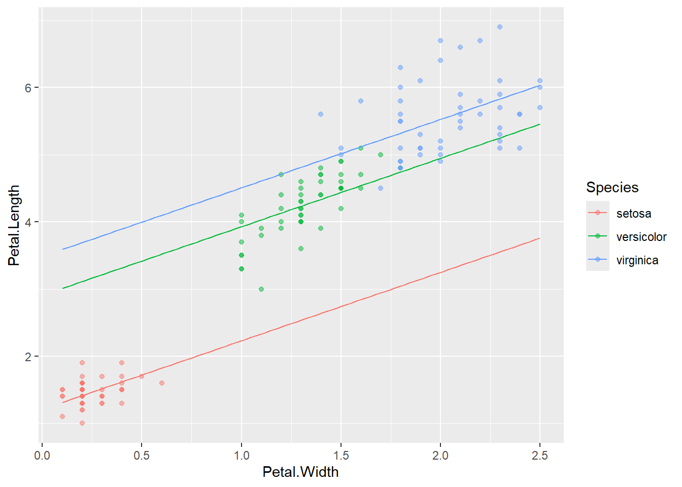

Figure 13.1: Example of model fitting to iris data. Points are observations, and lines are model predictions.

13.2.2 iris Example - interactive effects

In statistical models, an interaction occurs when the effect of one factor depends on the level of another factor. In the iris dataset, for example, the relationship between Petal.Length and Petal.Width may depend on species. We can represent this scenario with the following model:

# develop iris model with an interaction
m_iris_int <- lm(Petal.Length ~ Petal.Width * Species,
                 data = iris)

summary(m_iris_int)

## 
## Call:
## lm(formula = Petal.Length ~ Petal.Width * Species, data = iris)
## 
## Residuals:
##      Min       1Q   Median       3Q      Max 
## -0.84099 -0.19343 -0.03686  0.16314  1.17065 
## 
## Coefficients:
##                               Estimate Std. Error t value Pr(>|t|)    
## (Intercept)                     1.3276     0.1309  10.139  < 2e-16 ***
## Petal.Width                     0.5465     0.4900   1.115   0.2666    
## Speciesversicolor               0.4537     0.3737   1.214   0.2267    
## Speciesvirginica                2.9131     0.4060   7.175 3.53e-11 ***
## Petal.Width:Speciesversicolor   1.3228     0.5552   2.382   0.0185 *  
## Petal.Width:Speciesvirginica    0.1008     0.5248   0.192   0.8480    
## ---
## Signif. codes:  0 '***' 0.001 '**' 0.01 '*' 0.05 '.' 0.1 ' ' 1
## 
## Residual standard error: 0.3615 on 144 degrees of freedom
## Multiple R-squared:  0.9595, Adjusted R-squared:  0.9581 
## F-statistic: 681.9 on 5 and 144 DF,  p-value: < 2.2e-16

In this model:

• Petal.Width represents the effect of petal width on petal length for the reference species (setosa).

• Species captures differences in petal length among species when Petal.Width = 0.

• The interaction term (Petal.Width:Species) allows the slope of Petal.Length vs. Petal.Width to vary by species, meaning the effect of petal width can differ across species.

If the interaction term is significant, it indicates that the relationship between Petal.Length and Petal.Width depends on species, and visualizing the fitted lines for each species is helpful for interpretation.

# recreate prdiction dataframe
n_rep <- 100
df_pred <- iris %>% 
  group_by(Species) %>% 
  reframe(Petal.Width = seq(min(Petal.Width),
                            max(Petal.Width),
                            length = n_rep))

# prediction with the interaction model
y_pred_int <- predict(m_iris_int,
                      newdata = df_pred)

df_pred <- df_pred %>% 
  mutate(y_pred_int = y_pred_int)

# visualization
iris %>% 
  ggplot(aes(x = Petal.Width,
             y = Petal.Length,
             color = Species)) +
  geom_point(alpha = 0.5) +
  geom_line(data = df_pred,
            aes(y = y_pred_int))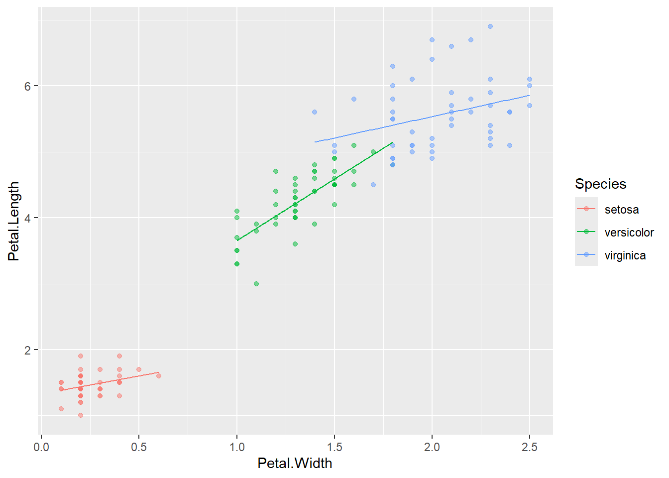

In this case, the interaction was significant for versicolor, and the slope is estimated to be clearly different from the other two.

13.2.3 Level of Measurament

1. Categorical Variables: Qualitative or discrete characteristics that fall into specific categories or groups. They do not have a numerical value or order associated with them. Examples: gender (male/female), marital status (single/married/divorced), and color (red/green/blue).

2. Ordinal Variables: Categories or levels with a natural order or ranking. Examples: survey ratings (e.g., Likert scale), education levels (e.g., high school, bachelor’s, master’s), or socioeconomic status (e.g., low, medium, high).

3. Interval Variables: Numerical values representing a continuous scale where the intervals between the values are meaningful and consistent. Unlike ordinal variables, interval variables have equally spaced intervals between adjacent values, allowing for meaningful arithmetic operations like addition and subtraction. However, interval variables do not contain a natural zero point; zero is arbitrary and merely a reference point. Examples: temperature

4. Ratio Variables: Numerical variable that shares the characteristics of interval variables but also has a meaningful and absolute zero point. Thus, this type of variables has the complete absence of the measured attribute/quantity. Examples: height (in centimeters), weight (in kilograms), time (in seconds), distance (in meters), and income (in dollars).

We cannot carry out meaningful arithmetic operations on categorical and ordinal variables; therefore, we should treat these variables as as “character” or “factors” in R. This is because R recognizes that the intervals between different groups or levels of these variables are not meaningful in a numerical sense.

In contrast, interval and ratio variables should be considered “numerical” variables in R. These variables possess a meaningful numerical scale with equal intervals, and in the case of ratio variables, a true zero point.

13.3 Non-parametric method

When the assumptions of linear models (e.g., normality, equal variances) are not met, nonparametric methods can be used. These methods do not assume a specific probability distribution for the data and can provide valid inference even with skewed or ordinal data.

Examples for common cases:

Purpose	Parametric Method (Normal Data)	Nonparametric Alternative (Non-normal Data)
Compare two groups	t-test	Wilcoxon rank-sum test (Mann–Whitney U test) wilcox.test()
Compare more than two groups	ANOVA	Kruskal–Wallis test kruskal.test()

13.4 Laboratory

13.4.1 Normality Assumption

The dataset ToothGrowth comes from a Guinea pig experiment that tested how Vitamin C affects tooth growth. Each observation represents a single guinea pig.

The experiment compared:

• Two supplement types: orange juice (OJ) and ascorbic acid (VC)

• Three dose levels: 0.5, 1, and 2 mg/day

Using this dataset,

1. Develop a linear model examining the effect of supplement type (supp), dose (dose), and their interaction on tooth length (len). Assign the developed model to m_tooth.

2. The Linear Model framework assumes normality. To verify the validity of the normality assumption, we typically employ the Shapiro-Wilk test (shapiro.test() in R). Discuss whether the test should be applied to (1) the response variable or (2) model residuals. Then, apply the Shapiro-Wilk. Type ?shapiro.test in the R console to learn more about its usage.

13.4.2 Model Interpretation

Using m_tooth, create a figure illustrating the relationship between tooth length (len; y-axis) and dose (dose; x-axis), with color indicating supplement type (supp). Include both the observed and predicted values, similar to Figure 13.1.

Use the following data frame for prediction:

df_pred <- ToothGrowth %>%
  group_by(supp) %>%
  reframe(dose = seq(min(dose),
                     max(dose),
                     length = 100))

13.4.3 Multicollinearity

Copy and run the following code to create a simulated dataset:

## variance-covariance matrix
mv <- rbind(c(1, 0.9),
            c(0.9, 1))

## true regression coefficients
b <- c(0.05, 1.00)

## produce simulated data
set.seed(523)
X <- MASS::mvrnorm(100,
                   mu = c(0, 0),
                   Sigma = mv)

df_y <- tibble(x1 = X[,1],
               x2 = X[,2]) %>% 
  mutate(y = rnorm(nrow(.),
                   mean = 1 + b[1] * x1 + b[2] * x2))

1. Create Figures of Response vs. Predictors.

Using df_y, create the following figures:

• A scatter plot of y (y-axis) versus x1 (x-axis)

• A scatter plot of y (y-axis) versus x2 (x-axis)

Based on these plots, interpret the effects of x1 and x2 on y. Do x1 and x2 appear to have positive or negative influences on y?

2. Examining statistical effects of x1 and x2 on y.

Examine the statistical effects of x1 and x2 on y using the lm() function.
Suppose that x1 and x2 are factors that vary across samples. In this case, you want to account for the influence of one variable while assessing the effect of the other. To do so, include both predictors in a single linear model using the + operator. Discuss whether the statistical estimates of x1 and x2’s effects make sense.

3. Create a Figure of Predictor vs. Predictor.

Using df_y,

• Create a scatter plot of x1 and x2.

• Examine the Pearson’s correlation between x1 and x2 using a function cor(). (?cor() for its usage).

13.4.4 Experimental Design

You are designing an experiment to examine the effects of nutrient level and predation on prey fish growth. The proposed treatment combinations are:

• Low nutrient and predator present

• High nutrient and predator present

• High nutrient and predator absent

In addition, you plan to record the initial length of the prey fish (a continuous variable), as it may influence subsequent growth.

Question: Select the most appropriate statement regarding what this experiment can assess:

1. This experiment can capture the effects of nutrient, predation, and their interaction.

2. This experiment can capture the effects of nutrient and predation. However, the nutrient effect may be limited to the presence of predators, and the predator effect is limited to the high nutrient condition.

3. This experiment can capture the effects of nutrient and predation. Main effects can be assessed across all nutrient conditions.

4. This experiment cannot capture either main effects or the interaction.