9 Likelihood

In Chapter 8, we introduced non-normal distributions to represent count and proportional data. The glm() function was used to obtain parameter estimates, but how does this function achieve that? In reality, the least squares approach is only applicable to normal distributions. Therefore, we require an alternative approach to estimate parameters within the GLM framework. In this section, I will introduce the concept of likelihood as a fundamental principle for parameter estimation in the GLM framework.

9.1 Finding the “More Likely”

In the least squares method, our goal is to minimize the sum of squared errors, ensuring that the fitted model has the smallest deviation from the observed data points. However, this approach is not applicable to non-normal variables. In such cases, we need to rely on the “probability” of observing a data point or numerical value.

Let’s consider an example where we have count data, denoted as \(\pmb{y} = \{y_1, y_2, ..., y_N\}\). To simplify the matter, let’s focus on a specific data point, say \(y_1 = 3\). Assuming a Poisson distribution, we can calculate the probability of observing this particular value by using an arbitrary parameter value for the mean, denoted as \(\lambda\). To refresh our memory, we can refer back to the Poisson distribution discussed in Chapter 3.

\[ \Pr(y = k) = \frac{\lambda^{k}\exp(-\lambda)}{k!} \]

This equation represents the probability of the variable \(y\) taking a specific value \(k\). In our current example, we are interested in the case where \(k = 3\). By specifying a value for the mean parameter \(\lambda\), we can compute the probability associated with this value. Let’s try using \(\lambda = 3.5\) for this calculation:

\[ \Pr(y_1 = 3) = \frac{3.5^3 \exp(-3.5)}{3!} \approx 0.215 \]

We can calculate this with dpois() in R:

# dpois()
# the first argument is "k"
# the second argument is "lambda"
dpois(3, lambda = 3.5)

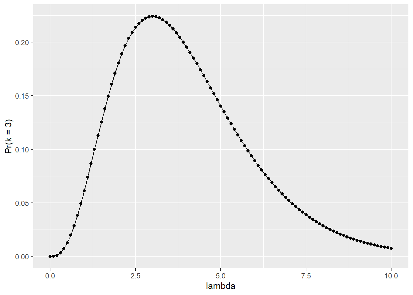
## [1] 0.2157855

# write the formula to confirm
(p <- (3.5^3 * exp(-3.5)) / factorial(3))

## [1] 0.2157855

If we assume a mean of \(3.5\) in the Poisson distribution, the probability of observing a value of \(3\) is approximately \(0.216\). We can experiment with different values of \(\lambda\) to see if there is a potentially “better” value. By exploring different values of \(\lambda\), we can observe how the probability of observing a specific value changes. This allows us to assess which value of \(\lambda\) provides a better fit or captures the data more accurately. The following example explores \(\lambda = 0 - 10\) with a \(0.1\) interval.

# change lambda from 0 to 10 by 0.1
lambda <- seq(0, 10, by = 0.1)

# probability
pr <- dpois(3, lambda = lambda)

# create a data frame
df_pois <- tibble(y = 3,
                  lambda = lambda,
                  pr = pr)

print(df_pois)

## # A tibble: 101 × 3
##        y lambda       pr
##    <dbl>  <dbl>    <dbl>
##  1     3    0   0       
##  2     3    0.1 0.000151
##  3     3    0.2 0.00109 
##  4     3    0.3 0.00333 
##  5     3    0.4 0.00715 
##  6     3    0.5 0.0126  
##  7     3    0.6 0.0198  
##  8     3    0.7 0.0284  
##  9     3    0.8 0.0383  
## 10     3    0.9 0.0494  
## # ℹ 91 more rows

Make a plot:

df_pois %>% 
  ggplot(aes(x = lambda,
             y = pr)) +
  geom_point() +
  geom_line() +
  labs(x = "lambda",
       y = "Pr(k = 3)")

Figure 9.1: Relationship between the parameter \(\lambda\) and the probability of observing a value of three.

By examining the figure or data, it appears that the probability is highest around \(\lambda = 3\). To confirm this observation, let’s arrange the data frame df_pois.

# arrange() re-orders the dataframe based on the speficied column in an ascending order
# desc() flips the order (descending)

df_pois %>% 
  arrange(desc(pr)) %>% 
  print()

## # A tibble: 101 × 3
##        y lambda    pr
##    <dbl>  <dbl> <dbl>
##  1     3    3   0.224
##  2     3    3.1 0.224
##  3     3    2.9 0.224
##  4     3    3.2 0.223
##  5     3    2.8 0.222
##  6     3    3.3 0.221
##  7     3    2.7 0.220
##  8     3    3.4 0.219
##  9     3    2.6 0.218
## 10     3    3.5 0.216
## # ℹ 91 more rows

That reasoning is sound because the probability of \(y_1\) being equal to \(3\) is maximized when \(\lambda = 3\). This represents the simplest form of a likelihood function denoted as \(L(\lambda~|~y_1)\), where \((\cdot~|~y_1)\) indicates that \(y_1\) is fixed or given. We evaluated the likelihood of various \(\lambda\) considering the given value of \(y_1\).

However, what if we have multiple values of \(y_i\)? Let’s consider the scenario where \(\pmb{y} = \{3, 2, 5\}\). In such cases, we must account for the probability of simultaneously observing these values. When the events are independent, the probability of observing multiple events can be expressed as the product of their individual probabilities. Consequently, the likelihood function takes the following form:

\[ \begin{aligned} L(\lambda~|~\pmb{y}) &= \Pr(y_1 = 3) \times \Pr(y_2 = 2) \times \Pr(y_3 = 5)\\ &= \frac{\lambda^{3}\exp(-\lambda)}{3!} \times \frac{\lambda^{2}\exp(-\lambda)}{2!} \times \frac{\lambda^{5}\exp(-\lambda)}{5!}\\ &= \prod_i^3 \frac{\lambda^{y_i} \exp(-\lambda)}{y_i!} \end{aligned} \]

Implement this in R:

# try lambda = 3 for y = 3, 2, 5
pr <- dpois(c(3, 2, 5), lambda = 3)
print(pr)

## [1] 0.2240418 0.2240418 0.1008188

# probability of observing 3, 2, 5 simultaneously
# with lambda = 3
prod(pr)

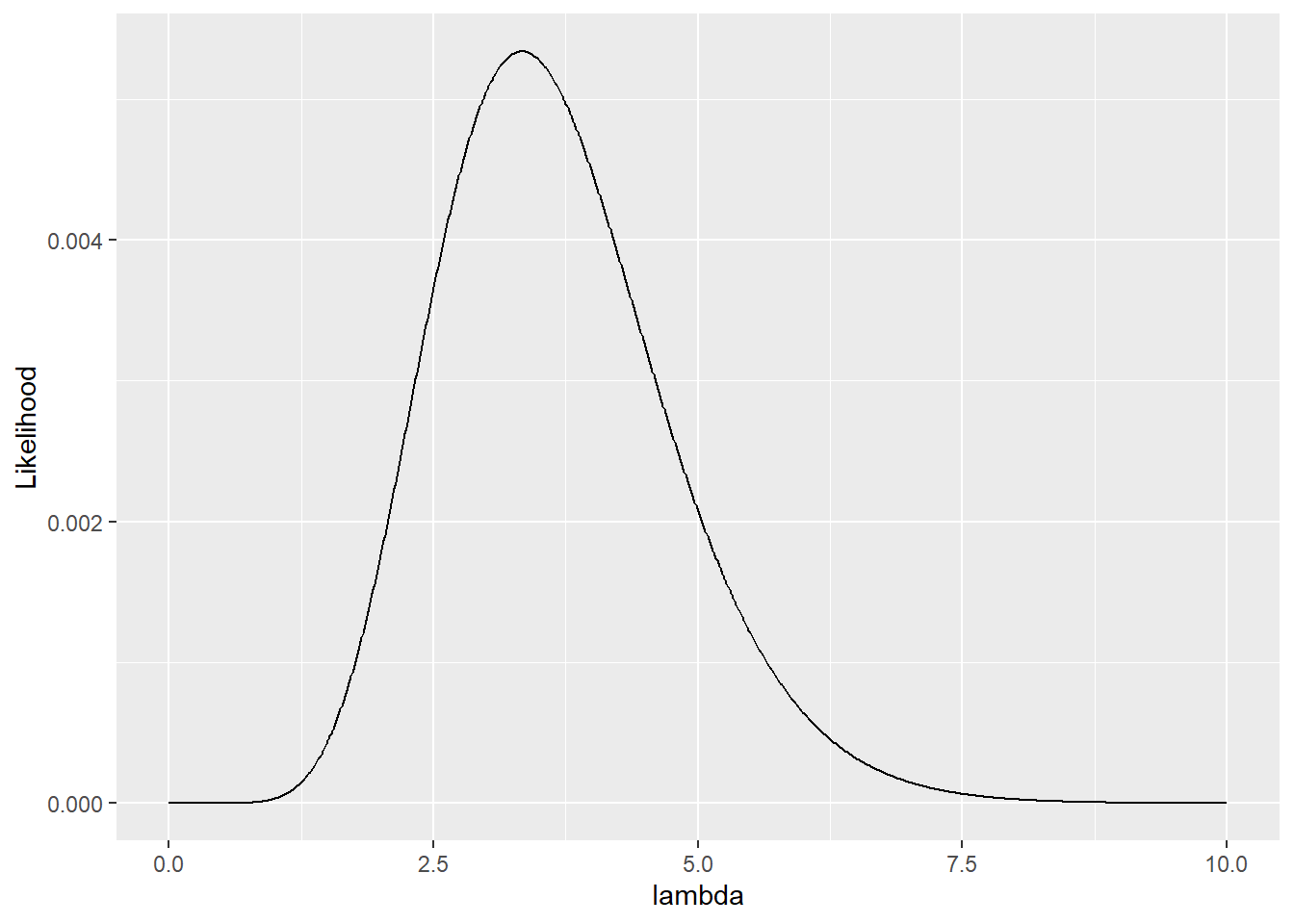
## [1] 0.005060573

Similar to the previous example, let’s search for a more suitable value of \(\lambda\) that better captures the observed data.

# lambda = 0 - 10 by 0.01
y <- c(3, 2, 5)
lambda <- seq(0, 10, by = 0.01)

# sapply repeats the task in FUN
# each element in "X" will be sequencially substituted in "z"
pr <- sapply(X = lambda,
             FUN = function(z) prod(dpois(y, lambda = z)))

# make a data frame and arrange by pr (likelihood)
df_pois <- tibble(lambda = lambda,
                  pr = pr)

df_pois %>% 
  arrange(desc(pr)) %>% 
  print()

## # A tibble: 1,001 × 2
##    lambda      pr
##     <dbl>   <dbl>
##  1   3.33 0.00534
##  2   3.34 0.00534
##  3   3.32 0.00534
##  4   3.35 0.00534
##  5   3.31 0.00534
##  6   3.36 0.00534
##  7   3.3  0.00534
##  8   3.37 0.00534
##  9   3.29 0.00533
## 10   3.38 0.00533
## # ℹ 991 more rows

# visualize
df_pois %>% 
  ggplot(aes(x = lambda,
             y = pr)) +
  geom_line() +
  labs(y = "Likelihood")

Figure 9.2: Likelihood of observing three count data points \(\pmb{y}\) simultaneously.

In this exercise with an interval of \(0.01\), \(\lambda \approx 3.33\) is identified as the most suitable value. Interestingly, the sample mean matches this value:

mean(c(3, 2, 5))

## [1] 3.333333

Why? See below.

9.2 Maximum Likelihood Method

9.2.1 Simple case

Finding the parameter value that maximizes the probability of observing a set of observed values is known as the Maximum Likelihood Estimate (MLE). This estimation method is commonly employed in the GLM framework and various other statistical inference techniques. The MLE approach is applicable as long as the likelihood can be defined, making it a versatile method for many statistical analyses.

However, the procedure I employed in the previous section (Section 9.1) is not mathematically rigorous because the optimal value of \(\lambda\) is dependent on the resolution of the interval. As the interval becomes smaller, it is possible to discover an even better value of \(\lambda\) ad infinitum due to its continuous nature.

A more reliable approach to identifying the “peak” is by utilizing the first-order derivative. The first-order derivative represents the slope of the likelihood function at a given \(\lambda\) value. If the derivative equals zero, it indicates that we have reached the peak of the likelihood function. We can leverage this mathematical principle to determine the maximum likelihood estimate of \(\lambda\). Since computing the derivative of a product is mathematically challenging, we can apply a logarithm transformation to the likelihood function. Recall that \(\log ab = \log a + \log b\). By taking the logarithm, we can convert the product operation \(\prod\) into a summation operation \(\sum\). Specifically:

\[ \begin{aligned} \log L(\lambda | \pmb{y}) &= \log \prod_i^N \frac{\lambda^{y_i} \exp(-\lambda)}{y_i!}\\ &= \log \frac{\lambda^{y_1} \exp(-\lambda)}{y_1!} + \log \frac{\lambda^{y_2} \exp(-\lambda)}{y_2!} + ... + \log \frac{\lambda^{y_N} \exp(-\lambda)}{y_N!}\\ &= \sum_i^N \log \frac{\lambda^{y_i} \exp(-\lambda)}{y_i!}\\ &= \sum_i^N (y_i \log \lambda -\lambda -\log y_i!) \end{aligned} \]

Taking the first derivative of \(\log L(\lambda | \pmb{y})\):

\[ \begin{aligned} \frac{\partial\log L(\lambda|\pmb{y})}{\partial \lambda} &= \sum_i^N (\frac{y_i}{\lambda} -1)\\ &= \frac{\sum_i^N y_i}{\lambda} - \sum_i^N 1\\ &= \frac{\sum_i^N y_i}{\lambda} - N\\ \end{aligned} \] To obtain the value of \(\lambda\) that maximizes the likelihood, we set the derivative equal to zero:

\[ \begin{aligned} \frac{\partial\log L(\lambda|\pmb{y})}{\partial \lambda} &= \frac{\sum_i^N y_i}{\lambda} - N = 0\\ \lambda &= \frac{\sum_i^N y_i}{N} \end{aligned} \]

Interesting – the maximum likelihood estimate of \(\lambda\) is equal to the sample mean. This is THE reason why we could use the sample mean as the estimate of \(\lambda\) in Chapter 3.

9.2.2 General case

In practice, obtaining the MLE analytically can be highly complex and often infeasible. Consequently, the GLM framework relies on numerical search algorithms to approximate the MLE estimates (see Ben Bolker’s book chapter for full details; in particular, quasi-Newton methods). Within GLMs, it is common to establish relationships between the mean \(\lambda\) and explanatory variables in order to investigate their influences. For instance:

\[ \begin{aligned} y_i &\sim \mbox{Poisson}(\lambda_i)\\ \log(\lambda_i) &= \alpha + \sum_k \beta_k x_k \end{aligned} \]

where \(x_k\) represents \(k\)th explanatory variable. This translates into:

\[ \log L(\alpha, \beta_1,...\beta_k|\pmb{y}) = \sum_i \left[y_i (\alpha + \sum_k\beta_k x_k) - \exp(\alpha + \sum_k \beta_k x_k) - \log y_i! \right] \]

and solving the \(k+1\) partial derivatives:

\[ \begin{aligned} \frac{\partial \log L(\alpha, \beta_1,...\beta_k|\pmb{y})}{\partial \alpha} &= 0\\ \frac{\partial \log L(\alpha, \beta_1,...\beta_k|\pmb{y})}{\partial \beta_1} &= 0\\ &...\\ \frac{\partial \log L(\alpha, \beta_1,...\beta_k|\pmb{y})}{\partial \beta_k} &= 0\\ \end{aligned} \]Thus, the function glm() does a lot for us! The log likelihood of the fitted model can be extracted with logLik():

# load garden plant data
# df_count <- read_csv("data_raw/data_garden_count.csv")

m_pois <- glm(count ~ nitrate,
              data = df_count,
              family = "poisson")

logLik(m_pois)

## 'log Lik.' -44.92912 (df=2)

9.3 Laboratory

9.3.1 Binomial Distribution

The binomial distribution is a probability distribution that describes the number of successes in a fixed number of independent Bernoulli trials, where each trial has the same probability of success, denoted by \(p\). The probability mass function (PMF) of a binomial distribution is given by:

\[ \Pr(y = k) = \begin{pmatrix} N\\ k \end{pmatrix} p^k(1 - p)^{N-k} \]

where \(\begin{pmatrix} N\\ k \end{pmatrix}\) is the binomial coefficient, representing the number of ways to choose \(k\) successes out of \(N\) trials.

1. The function dbinom() calculates \(\Pr(y = k)\) for a binomial distribution. Using this function, calculate the likelihood of observing the vector \(\pmb{y} = \{2, 2, 0, 0, 3, 1, 3, 3, 4, 3\}\) for the following values of \(p\): \(p \in \{0, 0.01, 0.02, ..., 1.0\}\), where \(N = 10\).

2. From the set of \(p\) examined, find the parameter value that maximizes the likelihood.

3. Using the \(p\) that maximizes the likelihood, calculate \(N \times p\). Compare this value with the sample mean of the vector \(\pmb{y}\).

9.3.2 Normal Distribution

The normal distribution is a continuous probability distribution that describes the distribution of a continuous random variable. It is characterized by its mean \(\mu\) and standard deviation \(\sigma\). The probability density function (PDF) of a normal distribution is given by:

\[ f(y) = \frac{1}{\sqrt{2 \pi} \sigma} \exp\left(-\frac{(y - \mu)^2}{2 \sigma^2}\right) \]

As the normal distribution deals with continuous variables, the PDF returns probability density instead of probability. However, we can define the likelihood of observing the entire vector \(\pmb{y}\) in a similar way:

\[ L(\mu, \sigma | \pmb{y}) = \prod_{i}^N f(y_i) \]

1. Yield the logarithm of \(L(\mu, \sigma | \pmb{y})\).

2. Derive the first-order derivative of the log-likelihood function with respect to \(\mu\) and solve for \(\mu\) by setting \(\frac{\partial \log L(\mu, \sigma)}{\partial \mu} = 0\). Assume \(\sigma\) is a constant.