20 Constrained Ordination

In unconstrained ordination, the axes are derived solely from the multivariate response data, without reference to external predictors. These methods are useful for exploring dominant patterns, visualizing similarity among samples, and generating hypotheses.

In many biological studies, however, we are explicitly interested in how external variables structure multivariate responses—for example, how species composition changes along gradients of moisture, land use, or management. Constrained ordination methods address this question by restricting the ordination axes to be linear (or unimodal) combinations of measured explanatory variables. In this sense, constrained ordination can be viewed as a multivariate extension of regression.

Learning Objectives:

• Understand the conceptual difference between unconstrained and constrained ordination.

• Apply constrained ordination methods (RDA, CCA, dbRDA) to relate multivariate responses to environmental predictors.

• Interpret constrained ordination diagrams, including site scores, species scores, and environmental vectors.

• Quantify and test the proportion of multivariate variation explained by predictors using permutation tests.

pacman::p_load(tidyverse,
               GGally,
               vegan)

20.1 Methods for Constrained Ordination

In constrained ordination, the term “constrained” refers to the fact that the ordination axes are determined by the explanatory variables, rather than emerging solely from the multivariate response data.

• The axes represent linear (or unimodal) combinations of measured predictors.

• Point coordinates in the ordination are interpretable in terms of these predictors.

These points contrast with unconstrained ordination, where axes summarize the total variation in the response data without reference to external variables.

The effects of predictors are estimated by identifying axes that maximize the variation in the multivariate response explained by the predictors. Mathematically, constrained ordination decomposes the total variation in the response matrix into the portion explained by the predictors and residual variation, with successive axes capturing the maximum remaining explained variation.

20.1.1 RDA

Lichen pasture

We will begin by the Redundancy Analysis (RDA), which is a constrained version of Principal Component Analysis (PCA). To illustrate a use case of RDA, we will use the varespec dataset. This dataset contains observations from 24 sampling sites (rows), with each column representing the estimated cover of one of 44 plant species (lichen, bryophytes, and vascular plants) at those sites. It comes with varechme data, which include 14 variables that summarize soil properties, such as nutrient concentrations and physical characteristics.

Before proceeding with the analysis, we will perform some basic data cleaning to ensure the datasets are easy to work with and consistently formatted.

# Load example datasets from the vegan package
data("varespec")  # Species abundance matrix: plant species measured at 44 sites
data("varechem")  # Environmental variables (soil chemistry) for the same sites

# Response matrix: species abundances
m_y <- varespec

# Convert column names to lowercase for consistency
# This avoids issues with formulas or later data manipulation
colnames(m_y) <- str_to_lower(colnames(varespec))

# Clean and prepare environmental data
# - Convert to tibble for easier use with dplyr
# - Use janitor::clean_names() to make column names lowercase, consistent, and safe for programming
df_env <- as_tibble(varechem) %>% 
  janitor::clean_names()

Visualization highlights the non-normal distributional patterns that are common in biological datasets.

# Pairwise scatterplot matrix of the first 3 species columns in m_y
m_y %>%
  ggpairs(
    progress = FALSE,      # Disable the progress bar during plotting
    columns = 1:3,         # Only use the first 3 species for the plot
    aes(
      alpha = 0.5           # Make points semi-transparent to reduce overplotting
    )
  ) +
  theme_bw()               # Use a clean theme with white background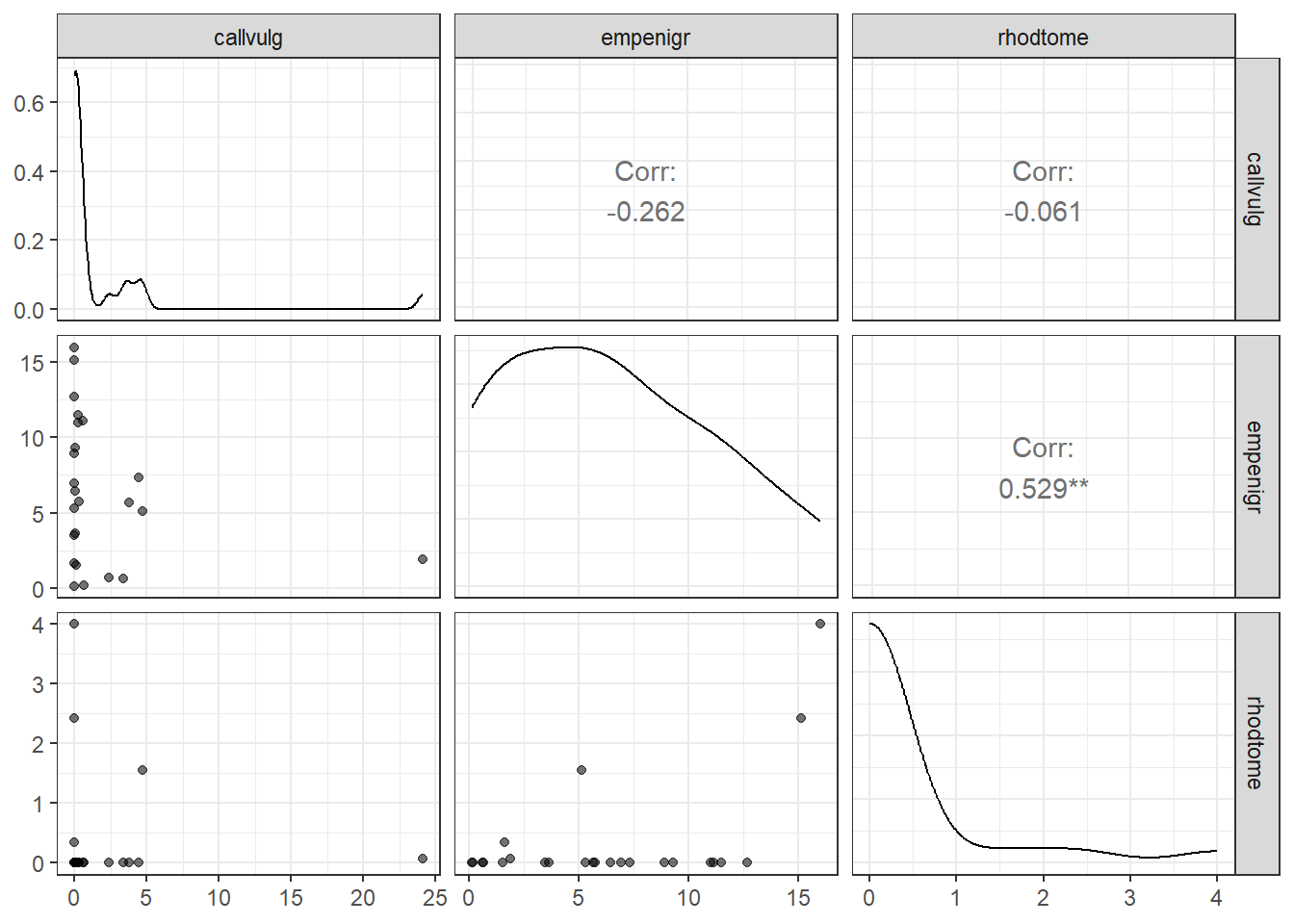

Performing RDA is straightforward, as the vegan package provides the rda() function for implementing this analysis. In the example below, we set scale = FALSE (default in rda()) because the response variables are already standardized as percent cover. If the variables were measured in different units (e.g., grams vs. meters) or differ grearly in their variations, scale = TRUE would be necessary to ensure that all variables contribute equally to the analysis.

# Run Redundancy Analysis (RDA)
# - Response: m_y (species abundance matrix, varespec)
#   Note: Hellinger transformation is recommended for raw species counts.
# - Predictors: n, p, k, ca (numeric soil chemistry variables from df_env)
#   These represent Nitrogen (n), Phosphorus (p), Potassium (k), and Calcium (ca) levels.
# - Data: df_env (cleaned environmental variables)
# The parentheses around obj_rda print the RDA summary immediately
(obj_rda <- rda(m_y ~ n + p + k + ca,
                data = df_env))

## Call: rda(formula = m_y ~ n + p + k + ca, data = df_env)
## 
##                 Inertia Proportion Rank
## Total         1825.6594     1.0000     
## Constrained    516.1041     0.2827    4
## Unconstrained 1309.5553     0.7173   19
## Inertia is variance 
## 
## Eigenvalues for constrained axes:
##   RDA1   RDA2   RDA3   RDA4 
## 244.71 216.40  30.61  24.37 
## 
## Eigenvalues for unconstrained axes:
##   PC1   PC2   PC3   PC4   PC5   PC6   PC7   PC8 
## 752.9 266.1 109.3  65.4  33.2  27.1  19.4  12.4 
## (Showing 8 of 19 unconstrained eigenvalues)

The RDA results show that the total variance (inertia) in the species abundance data is 1825.66, of which 28.3% (516.10) is explained by the four soil chemistry predictors (n, p, k, ca) and 71.7% (1309.56) remains unexplained (residual variation).

The first two axes of RDA axes (constrained) captured most of the explained variation, with eigenvalues of 244.71 (RDA1), 216.40 (RDA2), 30.61 (RDA3), and 24.37 (RDA4). The unconstrained axes, representing residual variation, have larger eigenvalues (e.g., PC1 = 752.9, PC2 = 266.1), showing that most variation in species composition is not accounted for by the measured soil variables.

Overall, this indicates that while soil chemistry influences species distributions, a substantial proportion of multivariate variation is structured by other unmeasured factors or stochastic processes.

However, we may be interested in the individual contribution of each predictor, particularly whether those contributions are statistically significant. To assess this, we can use the anova.cca() function from the vegan package, which performs permutation-based significance tests for constrained ordination models.

# Perform permutation test on the RDA object
# - obj_rda: RDA object containing species (response) and soil chemistry (predictors)
# - by = "margin": test the marginal effect of each predictor
#   This evaluates how much variation each predictor explains **after accounting for all other predictors**
# - permutations = 999: number of random permutations used to generate the null distribution for the F-statistic
anova.cca(obj_rda, 
          by = "margin", 
          permutations = 999)

## Permutation test for rda under reduced model
## Marginal effects of terms
## Permutation: free
## Number of permutations: 999
## 
## Model: rda(formula = m_y ~ n + p + k + ca, data = df_env)
##          Df Variance      F Pr(>F)  
## n         1   189.63 2.7512  0.048 *
## p         1    70.69 1.0256  0.370  
## k         1    40.41 0.5863  0.649  
## ca        1    80.83 1.1728  0.286  
## Residual 19  1309.56                
## ---
## Signif. codes:  0 '***' 0.001 '**' 0.01 '*' 0.05 '.' 0.1 ' ' 1

It is important to set by = "margin" when your goal is to assess the individual contribution of each predictor. An alternative option is by = "terms", but this corresponds to a method analogous to Type I ANOVA, where predictors are tested sequentially in the order they appear in the model formula. As a result, the order of predictors matters: for example, specifying m_y ~ n + p + k + ca versus m_y ~ p + n + k + ca can lead to different test results, because each predictor is evaluated after accounting only for those entered before it.

In contrast, setting by = "margin" invokes a procedure analogous to Type II ANOVA. Here, the effect of each predictor is tested after accounting for all other predictors in the model, regardless of their order in the formula. This approach is generally preferred when predictors are not strictly hierarchical and when the goal is to evaluate the unique contribution of each environmental variable to the multivariate response.

Horseshoe effect

Since RDA is based on PCA, it implicitly assumes linear relationships among the response variables. This assumption is often violated in typical biological datasets, as we see here. This example illustrates how RDA can be inappropriate for many biological response data, which are frequently non-normal and non-linearly related. RDA tends to perform better with variables that are approximately normally distributed and linearly related, such as physical measurements (e.g., temperature, water depth) or certain biological traits (e.g., body size).

When applied to non-linear data, visualization of the RDA axes can reveal artifacts such as the horseshoe effect, a mathematical distortion that arises when non-linear relationships are inappropriately treated as linear.

# Extract site (sample) scores from the RDA object
# - display = "sites": returns the coordinates of sampling sites in RDA space
# - scaling = 2: correlation scaling, which emphasizes relationships between sites
#   and explanatory variables (i.e., how site positions correlate with predictors)
# The site scores are then combined with the environmental data for visualization
df_rda <- scores(obj_rda, 
                 display = "sites",
                 scaling = 2) %>% 
  bind_cols(df_env) %>%           # append environmental variables (e.g., soil chemistry)
  janitor::clean_names()          # standardize column names for tidy workflows

# Create a ggplot2 ordination plot
# - Points represent sites positioned by their constrained community composition
# - Color gradient reflects the nitrogen (n) concentration at each site
df_rda %>% 
  ggplot(aes(x = rda1,
             y = rda2,
             color = n)) +        # color sites by nitrogen level
  geom_point() +
  theme_bw() +
  labs(x = "RDA1",
       y = "RDA2",
       color = "Nitrogen") +
  scale_color_viridis_c()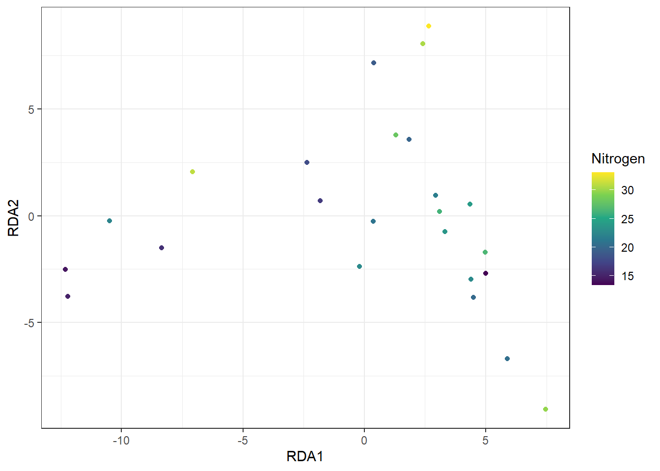

Figure 20.1: RDA ordination plot of sites based on species composition. Each point represents a site, positioned by its RDA scores (RDA1 and RDA2), with the color gradient indicating soil nitrogen (n) concentration, illustrating how environmental variation is associated with multivariate community patterns.

The plot clearly shows a unimodal pattern (“horseshoe”) along the RDA1 axis, which does not reflect a true biological pattern in the data. When such a pattern appears, it indicates that RDA—or any ordination method that assumes linear relationships—may be inappropriate; any statistical inference drawn from the results could be strongly biased.

20.1.2 dbRDA

While RDA provides an important extension of PCA to include environmental predictors, it also has limitations, particularly when species responses are non-linear or data are non-normal. To address this, we will explore distance-based RDA (dbRDA) as a more flexible alternative for constrained ordination.

Although dbRDA is not as flexible as NMDS, it allows the use of a distance or dissimilarity matrix as the response input instead of the raw data, greatly expanding its applicability to biological datasets with non-linear relationships.

The implementation requires only minimal changes. We can still use m_y from the previous example, but instead of rda(), we apply the capscale() function with distance = "bray". This internally converts the raw community matrix into a Bray-Curtis dissimilarity matrix, allowing distance-based constrained ordination.

# Perform distance-based Redundancy Analysis (dbRDA)
# - Response: m_y (species abundance matrix)
# - Predictors: n, p, k, ca (environmental variables: nitrogen, phosphorus, potassium, calcium)
# - data = df_env: provides the environmental variables used as predictors
# - distance = "bray": computes a Bray-Curtis dissimilarity matrix from the raw species abundances
#   internally, before performing the constrained ordination
# The result is a capscale object representing the constrained ordination in distance space
(obj_db <- dbrda(m_y ~ n + p + k + ca,
                 data = df_env,
                 distance = "bray"))

## Call: dbrda(formula = m_y ~ n + p + k + ca, data = df_env, distance =
## "bray")
## 
##               Inertia Proportion Rank RealDims
## Total           4.544      1.000              
## Constrained     1.164      0.256    4        4
## Unconstrained   3.381      0.744   19       14
## Inertia is squared Bray distance 
## 
## Eigenvalues for constrained axes:
## dbRDA1 dbRDA2 dbRDA3 dbRDA4 
## 0.5896 0.3408 0.1298 0.1034 
## 
## Eigenvalues for unconstrained axes:
##   MDS1   MDS2   MDS3   MDS4   MDS5   MDS6   MDS7   MDS8 
## 1.3418 0.7788 0.3983 0.2858 0.1825 0.1617 0.1186 0.0931 
## (Showing 8 of 19 unconstrained eigenvalues)

The interpretation is analogous to RDA. The total inertia represents the overall variation in Bray-Curtis dissimilarity among sites. The constrained inertia (1.197) indicates that about 26% of the total variation in species composition is explained by the environmental predictors (n, p, k, ca), with the remaining variation (3.606) unconstrained or residual.

The eigenvalues for the constrained axes (dbRDA1 – dbRDA4) indicate how much of the explained variation each axis captures, while the unconstrained axes (MDS1–MDS15) summarize the residual variation in distance space.

Although the output resembles RDA, an important distinction is that dbRDA operates on a distance matrix, rather than raw biological data (in this case, percent cover), allowing it to accommodate non-linear and non-Euclidean relationships. In this way, dbRDA extends RDA to more complex biological datasets, providing a flexible framework for constrained ordination when linear assumptions are not met.

Re-running the permutation test produces a contrasting result for soil nitrogen, which is now neither statistically significant nor marginally significant. This highlights the importance of carefully assessing the properties of your data before applying linear ordination methods, as assumptions violations can strongly affect statistical inference.

# Perform a permutation test on the dbRDA object
# - obj_db: the dbRDA (dbrda) object containing species distances and predictors
# - by = "margin": tests the **marginal effect** of each predictor, i.e., the unique contribution
#   of a variable after accounting for all other predictors in the model
# - permutations = 999: randomly permutes the data 999 times to generate a null distribution
#   for the F-statistic, allowing assessment of statistical significance
anova.cca(obj_db,
          by = "margin",
          permutations = 999)

## Permutation test for dbrda under reduced model
## Marginal effects of terms
## Permutation: free
## Number of permutations: 999
## 
## Model: dbrda(formula = m_y ~ n + p + k + ca, data = df_env, distance = "bray")
##          Df SumOfSqs      F Pr(>F)
## n         1   0.2879 1.6177  0.136
## p         1   0.1529 0.8593  0.507
## k         1   0.1450 0.8150  0.581
## ca        1   0.2733 1.5357  0.162
## Residual 19   3.3809

We can now examine whether dbRDA has mitigated the horseshoe effect, reducing the distortions seen in linear RDA when species responses are non-linear.

# Extract site scores from the dbRDA object
# - display = "sites": retrieves the coordinates of each site in the constrained ordination space
# - scaling = 2: correlation (or "standardized") scaling, which emphasizes relationships between sites
#   and environmental predictors rather than absolute distances
# - as_tibble(): converts the site scores to a tibble for easier manipulation with dplyr
# - bind_cols(df_env): adds the original environmental variables for plotting, coloring, or annotation
# - janitor::clean_names(): ensures consistent, safe column names for programming

df_db <- scores(obj_db, 
                display = "sites",
                scaling = 2) %>% 
  as_tibble() %>%              
  bind_cols(df_env) %>%        
  janitor::clean_names()       

# Create a basic ggplot ordination plot
# - Each point represents a site in the dbRDA ordination space
# - Points can later be colored, shaped, or labeled by environmental variables for interpretation
df_db %>% 
  ggplot(aes(x = db_rda1,
             y = db_rda2)) +
  geom_point() +               # plot sites as points
  labs(x = "dbRDA1",
       y = "dbRDA2")

Figure 20.2: Scatterplot of sites in dbRDA space. Each point represents a site positioned according to its constrained ordination scores, summarizing variation in species composition explained by the environmental predictors.

20.1.3 Other Options

Like unconstrained ordination, there are various constrained ordination methods, each with different assumptions and levels of flexibility. Common approaches include RDA and dbRDA, which can be seen as two extremes: RDA assumes linear relationships and normally distributed response variables, while dbRDA allows non-Euclidean distances and non-linear relationships.

The most appropriate method depends on your data characteristics and analytical goals. Methods with stricter assumptions, like RDA, have limited applicability, but can provide more quantitative precision if the assumptions are met. More flexible methods, such as dbRDA or distance-based approaches, are widely applicable, but may sacrifice some quantitative detail in exchange for robustness to non-linear or non-normal data.

Method	Advantage	Limitation	Example Applications
RDA (Redundancy Analysis)	Extends PCA to include environmental predictors; quantitative axes	Assumes linear relationships; sensitive to non-normal or zero-inflated data; may produce artifacts (e.g., horseshoe effect) with long gradients	Continuous trait data, species abundance matrices with linear responses, environmental gradients
CCA (Canonical Correspondence Analysis)	Extends CA to include environmental predictors; models unimodal species responses; interpretable species–environment relationships	Assumes unimodal responses; sensitive to rare species; may still produce arch effects if gradient is extreme	Community ecology with count/abundance data, species–environment relationships along long ecological gradients
dbRDA / CAP (Distance-based RDA / Constrained Analysis of Principal Coordinates)	Uses distance or dissimilarity matrix; flexible with non-Euclidean distances; can handle non-linear relationships	Less quantitative than RDA in raw units; may produce small imaginary components; interpretation depends on distance metric	Ecological community data with many zeros or non-normal distributions, Bray-Curtis or Jaccard distances, functional or phylogenetic distance matrices