17 Generalized Linear Mixed Effect Model

In the previous chapters, we developed foundational skills in linear modeling, including generalized linear models (GLMs). GLMs are a powerful and flexible framework when data arise from a single, relatively homogeneous set of observational units. However, ecological and biological data are often structured into multiple groups that differ in their underlying characteristics (e.g., sites, individuals, years). When such hierarchical or grouped structure is present, generalized linear mixed-effects models (GLMMs) provide a natural extension of GLMs by explicitly accounting for both shared population-level effects and group-specific variation.

Learning Objectives:

• Understand group structure in biological data

• Understand random intercept and slope

• Understand when random effects are preferred over fixed effects

pacman::p_load(tidyverse,
               lme4,
               glmmTMB)

17.1 Group Structure

In ecological studies, data are often collected in a hierarchical or grouped structure rather than as independent observations. For example, measurements may be repeated across sites within watersheds, individuals within populations, or years within study locations.

Let’s use Owls dataset from the R package glmmTMB to grasp the idea of how it works. This dataset is originally published in Roulin and Bersier 2007, Animal Behavior.

data(Owls) # from `glmmTMB`

# convert Owls to tibble
df_owl_raw <- as_tibble(Owls)

This dataset contains observations on begging behavior of barn owl nestlings across different experimental conditions. The data come from a study investigating sibling negotiation—a vocal communication system where nestlings use calls to peacefully resolve which individual will receive the next food item delivered by parents.

The experiment manipulated hunger levels by either food-depriving or satiating nestlings, then recorded their negotiation calls during parental arrivals. This allowed researchers to test whether negotiation intensity honestly signals hunger and whether nestlings adjust their calling based on which parent (male or female) arrives at the nest. The dataset includes repeated observations across 27 nests over time, in each of which the researchers counted negotiation calls by individual chick - thus, the data has a group (or nested) structure (599 observations at the individual level, nested within 27 nests).

It has seven main columns:

• Nest, a factor identifying each of the 27 individual nests.

• FoodTreatment, indicating whether the nestlings were experimentally “Deprived” (kept hungry before observation) or “Satiated” (fed before observation).

• SexParent, identifying whether the provisioning parent was “Male” or “Female.”

• ArrivalTime, the time when the parent arrived at the nest.

• SiblingNegotiation, the number of negotiation calls made by siblings (the primary response variable).

• BroodSize, the number of chicks in the nest.

• NegPerChick, the number of negotiations per chick.

Since this original data contains a mix of upper- and lower-case letters, we will first clean the format:

df_owl <- df_owl_raw %>% 
  janitor::clean_names() %>% 
  mutate(across(.cols = where(is.factor), 
                .fns = str_to_lower)) # apply str_to_lower() if column data type is factor

print(colnames(df_owl))

## [1] "nest"                "food_treatment"      "sex_parent"         
## [4] "arrival_time"        "sibling_negotiation" "brood_size"         
## [7] "neg_per_chick"       "log_brood_size"

Then, visualize the data. Our primary interest here is whether food_treatment changed the number of negotiations per chick (neg_per_chick = sibling_negotiation / brood_size):

df_owl %>% 
  ggplot(aes(x = food_treatment,
             y = neg_per_chick)) +
  geom_boxplot(outliers = FALSE) +
  geom_jitter(alpha = 0.25) +
  theme_bw()

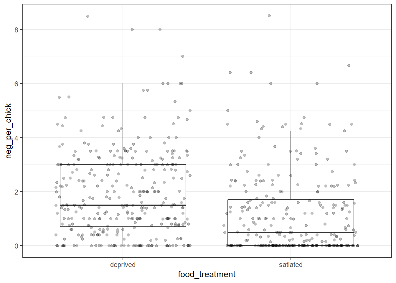
At first glance, the figure appears straightforward: the number of negotiations per chick decreases when nestlings are satiated. However, a closer examination reveals an important additional complexity in the data—its grouped structure. The example below highlights the first nine nests, illustrating substantial variation in neg_per_chick among nests.

# select the first nine groups
v_g9 <- unique(df_owl$nest)[1:9]

df_owl %>% 
  filter(nest %in% v_g9) %>% 
  ggplot(aes(x = food_treatment,
             y = neg_per_chick)) +
  geom_boxplot() +
  facet_wrap(facets =~ nest,
             ncol = 3,
             nrow = 3) +
  theme_bw()

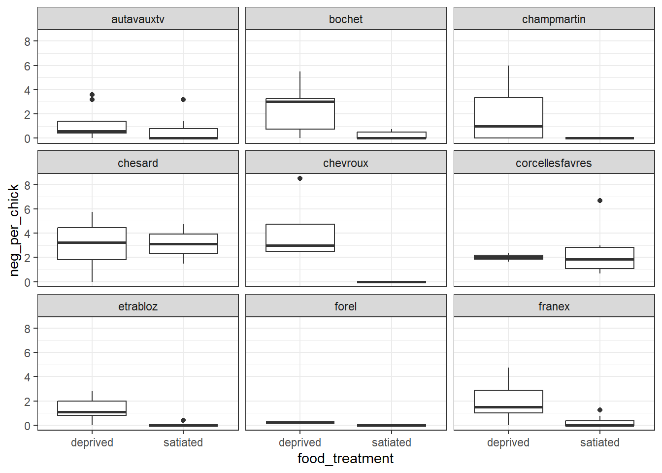
To examine the effect of food treatment while accounting for differences among nests, the GLM can be specified as follows:

# Response: sibling_negotiation — raw count of negotiation calls
# Predictors: food_treatment and nest
# Offset: log(brood_size)
# Note: Including this offset models the log rate of negotiations per chick,
#       i.e., log(sibling_negotiation / brood_size), which is equivalent to neg_per_chick

# check mean and variance of the response
# (mu_y <- mean(df_owl$sibling_negotiation)) # 6.72
# (var_y <- var(df_owl$sibling_negotiation)) # 44.50

# the response variable is count data
# variance >> mean
# choice of error distribution = negative-binomal
(m_glm <- MASS::glm.nb(sibling_negotiation ~ food_treatment + nest + offset(log(brood_size)),
                       data = df_owl))

## 
## Call:  MASS::glm.nb(formula = sibling_negotiation ~ food_treatment + 
##     nest + offset(log(brood_size)), data = df_owl, init.theta = 0.911083123, 
##     link = log)
## 
## Coefficients:
##            (Intercept)  food_treatmentsatiated              nestbochet  
##                0.20011                -0.78129                 0.20020  
##        nestchampmartin             nestchesard            nestchevroux  
##                0.14911                 1.02631                 0.44853  
##    nestcorcellesfavres            nestetrabloz               nestforel  
##                1.27423                -0.20826                -2.55492  
##             nestfranex                nestgdlv          nestgletterens  
##                0.31528                 0.24989                 0.74728  
##            nesthenniez               nestjeuss         nestlesplanches  
##                0.52213                -0.63986                 0.31026  
##             nestlucens               nestlully             nestmarnand  
##                0.53563                 0.83107                 0.56212  
##             nestmontet              nestmurist              nestoleyes  
##                0.66764                 1.01809                 0.71780  
##            nestpayerne              nestrueyes               nestseiry  
##                0.48422                 1.15510                 0.62465  
##              nestsevaz             neststaubin                nesttrey  
##                1.73558                 0.06776                 1.25416  
##           nestyvonnand  
##                0.62720  
## 
## Degrees of Freedom: 598 Total (i.e. Null);  571 Residual
## Null Deviance:       821.1 
## Residual Deviance: 705.4     AIC: 3477

Although this model works, it is not advisable. Because there are 27 nests, the model estimates 26 separate parameters, using the first nest as the reference category. This results in an unnecessarily complex model. More importantly, these nest-specific coefficients are not biologically interpretable: comparing one arbitrary nest (e.g., the first) to another does not provide meaningful biological insight, as the data do not encode specific biological differences among nests.

17.2 Random Intercept

17.2.1 Developing a model

Variables included as explicit predictors or explanatory variables are typically referred to as fixed effects. In the previous example, both food_treatment and nest were treated as fixed effects. Fixed effects are usually the primary focus of an analysis, as they represent factors whose effects we wish to estimate directly and interpret in a biological context.

However, as noted above, differences among nests are not biologically interpretable, making them inappropriate to include as fixed effects. At the same time, ignoring variation among nests altogether by excluding them from the model would bias the estimated effect of food_treatment.

Random effects are well suited to this situation. They represent categorical grouping variables that assign individual observations to a smaller number of groups. In the example above, nest is an ideal random effect because it groups individual chicks within nests, capturing among-nest variation without requiring explicit estimation of nest-specific effects.

Let’s develop a model that includes nest as a random effect. We will use the glmmTMB() function from the glmmTMB package, specifying the random effect with the syntax (1 | nest).

m_ri <- glmmTMB(sibling_negotiation ~ food_treatment + (1 | nest) + offset(log(brood_size)),
                 data = df_owl,
                 family = nbinom1()) # nbinom1() is from glmmTMB package

summary(m_ri)

##  Family: nbinom1  ( log )
## Formula:          
## sibling_negotiation ~ food_treatment + (1 | nest) + offset(log(brood_size))
## Data: df_owl
## 
##       AIC       BIC    logLik -2*log(L)  df.resid 
##    3398.3    3415.9   -1695.2    3390.3       595 
## 
## Random effects:
## 
## Conditional model:
##  Groups Name        Variance Std.Dev.
##  nest   (Intercept) 0.1303   0.361   
## Number of obs: 599, groups:  nest, 27
## 
## Dispersion parameter for nbinom1 family (): 7.05 
## 
## Conditional model:
##                        Estimate Std. Error z value Pr(>|z|)    
## (Intercept)             0.70686    0.09158   7.718 1.18e-14 ***
## food_treatmentsatiated -0.80409    0.08801  -9.137  < 2e-16 ***
## ---
## Signif. codes:  0 '***' 0.001 '**' 0.01 '*' 0.05 '.' 0.1 ' ' 1

Fixed effects still estimate (Intercept) and the effect of food_treatment. The key distinction from a standard GLM is that there are no nest-specific coefficients in the GLMM; instead, the model estimates the standard deviation of the nest effect (estimated as Std.Dev. 0.361), capturing among-nest variation.

The “trick” of GLMMs is to model only the variation between groups as a single random effect (one parameter), rather than estimating a separate parameter for each nest (26 parameters). This substantially reduces the number of parameters, improving model efficiency and increasing the reliability of estimated fixed effects.

17.2.2 Visualize model output

In a GLMM, random effects (e.g., nests, plots, or subjects) are modeled as variation among groups, summarized as a standard deviation in intercept rather than as separate fixed-effect parameters for each group. This means the model estimates how much groups vary around the overall mean, not individual group intercepts directly. We call this specification a random-intercept model because it allows group-specific intercepts.

You can obtain group-specific intercepts using coef() function:

head(coef(m_ri)$cond$nest)

##                 (Intercept) food_treatmentsatiated
## autavauxtv        0.3069198              -0.804093
## bochet            0.4859150              -0.804093
## champmartin       0.3868899              -0.804093
## chesard           1.1533443              -0.804093
## chevroux          0.7366369              -0.804093
## corcellesfavres   1.3333675              -0.804093

The returned values in (Intercept) represent group-specific intercepts, showing that GLMMs account for group-level variation by allowing the intercept to vary across groups. The coefficient of food_treatmentsatiated is constant across nests because we did not allow variation in this parameter among groups.

Since plotting all 27 nests would be tedious and hard to track visually, we will use only random nine nests for this exercise:

# ------------------------------------------------------------
# 1. Global (population-level) intercept on the response scale
# ------------------------------------------------------------
# The model uses a log link (negative binomial),
# so the intercept is on the log scale.
# We exponentiate it to return to the original response scale.
g0 <- exp(fixef(m_ri)$cond[1])


# ------------------------------------------------------------
# 2. Select a subset of nests to visualize
# ------------------------------------------------------------
# Plotting all 27 nests would be visually overwhelming,
# so we randomly select 9 nests for this example.
set.seed(123)  # ensures reproducibility
v_g9_ran <- sample(unique(df_owl$nest),
                   size = 9)


# ------------------------------------------------------------
# 3. Extract nest-specific coefficients (random intercept model)
# ------------------------------------------------------------
# coef(m_ri) returns the sum of fixed + random effects for each nest.
# These values are still on the log scale.
df_g9 <- coef(m_ri)$cond$nest %>% 
  as_tibble(rownames = "nest") %>%      # convert to tibble and keep nest ID
  filter(nest %in% v_g9_ran) %>%         # keep only the selected nests
  rename(
    log_g = `(Intercept)`,               # nest-specific intercept (log scale)
    b = food_treatmentsatiated            # fixed slope for food treatment
  ) %>% 
  mutate(
    g = exp(log_g),                      # intercept on response scale
    s = exp(log_g + b)                   # predicted value under satiated treatment
  )


# ------------------------------------------------------------
# 4. Create the figure
# ------------------------------------------------------------
df_owl %>% 
  filter(nest %in% v_g9_ran) %>%         # plot only the selected nests
  ggplot(aes(x = food_treatment,
             y = neg_per_chick)) +
  # Raw data points (jittered to reduce overlap)
  geom_jitter(width = 0.1,
              alpha = 0.5) +
  # Dashed horizontal lines:
  # nest-specific intercepts (baseline differences among nests)
  geom_hline(data = df_g9,
             aes(yintercept = g),
             alpha = 0.5,
             linetype = "dashed") +
  # Solid line segments:
  # predicted change from unfed to satiated treatment
  # using a common (fixed) slope across nests
  geom_segment(data = df_g9,
               aes(y = g,
                   yend = s,
                   x = 1,
                   xend = 2),
               linewidth = 0.5,
               linetype = "solid") +
  # Solid blue horizontal line:
  # global (population-level) intercept
  geom_hline(yintercept = g0,
             alpha = 0.5,
             linewidth = 1,
             linetype = "solid",
             color = "steelblue") +
  # Facet by nest to emphasize group-level structure
  facet_wrap(facets =~ nest,
             nrow = 3,
             ncol = 3) +
  theme_bw()

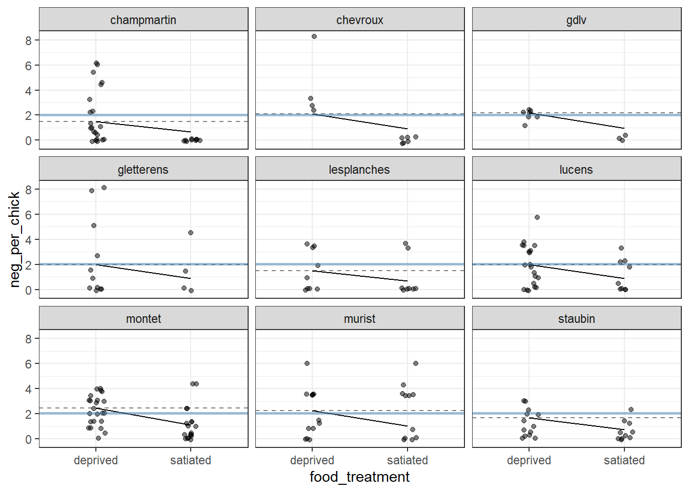
Figure 17.1: Visualization of a random‐intercept GLMM fitted to owl nesting data for a subset of nine nests. Points show observed counts of negotiation calls per chick. Dashed horizontal lines indicate nest‐specific intercepts (back‐transformed to the response scale from the log link), reflecting baseline differences among nests. Solid line segments connect predicted values under unfed and satiated treatments, illustrating the common (fixed) effect of food treatment, which is assumed to be identical across nests in the random‐intercept model. The solid blue horizontal line represents the global intercept (population‐level mean). Panels are faceted by nest to emphasize between‐nest variation in baseline response.

17.3 Random Intercept and Slope

17.3.1 Adding a random slope term

In the random-intercept model, written as (1 | nest) in the above example, we allow each nest to have its own baseline level (its own intercept) in the number of negotiations per chick. In other words, nests can start at different average values. However, as we saw from coef(m_ri), the effect of food_treatment is the same for all nests—the slope does not change across nests.

This reflects an assumption of the model: while nests may differ in their overall level, the effect of food treatment is assumed to be similar across nests. Any nest-to-nest differences in how food treatment works are assumed to be small enough to ignore.

We can relax this assumption by allowing the effect of food treatment to vary among nests. This is done by specifying the random effect as (1 + food_treatment | nest). In this random-intercept and random-slope model, the model still estimates an average effect of food treatment, but it also allows each nest to have its own slope, capturing differences in how strongly nests respond to the treatment:

m_ris <- glmmTMB(sibling_negotiation ~ food_treatment + (1 + food_treatment | nest) + offset(log(brood_size)),
                 data = df_owl,
                 family = nbinom1())

summary(m_ris)

##  Family: nbinom1  ( log )
## Formula:          sibling_negotiation ~ food_treatment + (1 + food_treatment |  
##     nest) + offset(log(brood_size))
## Data: df_owl
## 
##       AIC       BIC    logLik -2*log(L)  df.resid 
##    3375.0    3401.4   -1681.5    3363.0       593 
## 
## Random effects:
## 
## Conditional model:
##  Groups Name                   Variance Std.Dev. Corr 
##  nest   (Intercept)            0.03344  0.1829        
##         food_treatmentsatiated 0.45533  0.6748   0.98 
## Number of obs: 599, groups:  nest, 27
## 
## Dispersion parameter for nbinom1 family (): 6.69 
## 
## Conditional model:
##                        Estimate Std. Error z value Pr(>|z|)    
## (Intercept)              0.6871     0.0631  10.889  < 2e-16 ***
## food_treatmentsatiated  -0.9461     0.1697  -5.574  2.5e-08 ***
## ---
## Signif. codes:  0 '***' 0.001 '**' 0.01 '*' 0.05 '.' 0.1 ' ' 1

Now, coef(m_ris)$cond$nest returns variable slopes among nests, reflecting the assumption of the random slope:

head(coef(m_ris)$cond$nest)

##                 (Intercept) food_treatmentsatiated
## autavauxtv        0.5331993            -1.48889298
## bochet            0.5803105            -1.35054309
## champmartin       0.4398083            -1.87282147
## chesard           0.9839338             0.13947666
## chevroux          0.5679606            -1.40213486
## corcellesfavres   0.9386517            -0.01030472

Again, visualization helps clarify how this model differs from the random-intercept model. In the random-intercept case, lines for different nests are parallel, because the effect of food treatment is the same across nests.

The following code highlights how the effect of food treatment differs among nests by allowing each nest to have its own slope. As a result, the lines are no longer parallel, making it easy to see nest-specific responses to the food treatment.

# ------------------------------------------------------------
# 1. Extract nest-specific coefficients from the random-slope model
# ------------------------------------------------------------
# coef(m_ris) returns the sum of fixed + random effects for each nest.
# In this model, BOTH the intercept and the slope of food treatment
# are allowed to vary among nests.
# All coefficients are still on the log scale.
df_s9 <- coef(m_ris)$cond$nest %>% 
  as_tibble(rownames = "nest") %>%       # convert to tibble and keep nest ID
  rename(
    log_g = `(Intercept)`,               # nest-specific intercept (log scale)
    b = "food_treatmentsatiated"          # nest-specific slope (log scale)
  ) %>% 
  mutate(
    g = exp(log_g),                      # intercept on response scale
    s = exp(log_g + b)                   # predicted value under satiated treatment
  ) %>% 
  filter(nest %in% v_g9_ran)              # keep only the selected nine nests


# ------------------------------------------------------------
# 2. Create the figure
# ------------------------------------------------------------
df_owl %>% 
  filter(nest %in% v_g9_ran) %>%          # plot only the selected nests
  ggplot(aes(x = food_treatment,
             y = neg_per_chick)) +
  # Raw data points (jittered to reduce overlap)
  geom_jitter(width = 0.1,
              alpha = 0.5) +
  # DOTTED line segments:
  # predictions from the random-intercept model
  # (intercepts vary, but slopes are assumed identical across nests)
  geom_segment(data = df_g9,
               aes(y = g,
                   yend = s,
                   x = 1,
                   xend = 2),
               linewidth = 0.5,
               linetype = "dotted") +
  # SOLID line segments:
  # predictions from the random-intercept + random-slope model
  # both intercepts and slopes vary among nests
  # color represents the nest-specific slope estimate
  geom_segment(data = df_s9,
               aes(y = g,
                   yend = s,
                   x = 1,
                   xend = 2,
                   color = b),
               linewidth = 1,
               linetype = "solid") +
  # Solid blue horizontal line:
  # global (population-level) intercept
  geom_hline(yintercept = g0,
             alpha = 0.5,
             linewidth = 1,
             linetype = "solid",
             color = "steelblue") +
  # Facet by nest to highlight group-level heterogeneity
  facet_wrap(facets =~ nest,
             nrow = 3,
             ncol = 3) +
  theme_bw() +
  # Color scale for nest-specific slopes
  scale_color_viridis_c()

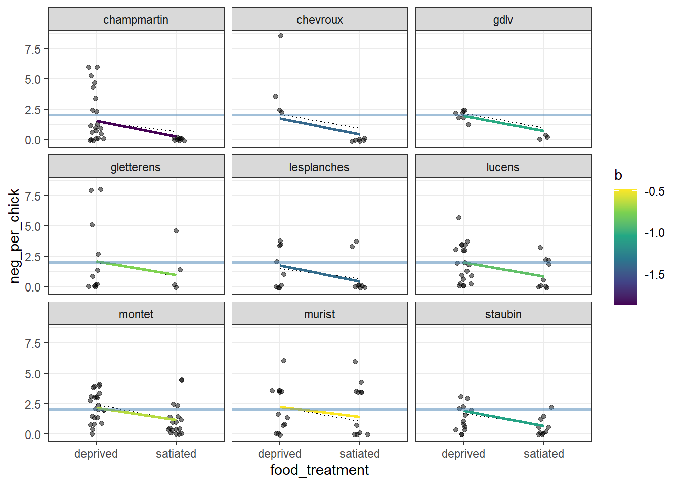
Figure 17.2: Visualization of a random‐intercept and random‐slope GLMM fitted to owl nesting data for a subset of nine nests. Points show observed counts of negotiation calls per chick under each food treatment. Dotted line segments represent predictions from the random‐intercept model, where the effect of food treatment is assumed to be constant across nests. Solid line segments show predictions from the random‐slope model, allowing the effect of food treatment to vary among nests; color indicates the nest‐specific slope estimate. The solid blue horizontal line denotes the global (population‐level) intercept. Panels are faceted by nest to emphasize differences in both baseline response and treatment effects.

17.4 Fixed vs Random

In statistical modeling, particularly in ecology, factors in a dataset can be treated as fixed effects or random effects. Choosing the appropriate type affects how we interpret model coefficients and account for variation in the data. Fixed effects are used when we are specifically interested in estimating and comparing the levels of a factor, while random effects are used when the levels represent a sample from a larger population and we are primarily interested in quantifying variability among them.

Type	Interpretation	Examples
Fixed effect	You are explicitly interested in the slope of specific levels of the factor or of continuous variable. Can be categorical or continuous.	Nutrient treatment (ambient vs. added), Sex (male vs. female), Temperature (continuous)
Random effect	The levels are a sample from a larger population. You are not interested in estimating each level, but rather in modeling variation among them. Must be categorical.	Nest ID, Site, Year, Block, Individual ID

17.5 Model specification

17.5.1 Rnadom intercept

With \(y_i\) denoting the number of negotiation calls (sibling_negotiation), the above example is formulated as follows:

\[ y_i \sim \mbox{NB}(\mu_i, \theta)\\ \ln \mu_i = \underbrace{(\alpha + \gamma_{j(i)})}_{\text{intercept + random effect term}} + \underbrace{\beta}_{\text{slope}} x_i + \ln(\mbox{offset term})\\ \gamma_j \sim \mbox{Normal}(0, \sigma_{\gamma}^2) \]

Here, \(i\) indexes individuals, and \(j(i)\) denotes the nest to which individual \(i\) belongs. In our model estimates, global intercept \(\alpha\) = 0.71, effect of food treatment \(\beta\) = -0.8, dispersion parameter \(\theta\) = 7.05, and SD of the random effect \(\sigma_{\gamma}\) = 0.13. Although this example uses a negative binomial model, the overall structure is similar for other probability distributions, provided an appropriate link function is chosen.

17.5.2 Random intercept and slope

With the random slope term, the model specification becomes:

\[ y_i \sim \mbox{NB}(\mu_i, \theta)\\ \ln \mu_i = \underbrace{(\alpha + \gamma_{j(i)})}_{\text{intercept + random effect term}} + \underbrace{(\beta + \delta_{j(i)})}_{\text{slope + random effect term}} x_i + \ln(\mbox{offset term})\\\]

When a random slope term is included, random intercept and slope terms are assumed to follow a multi-variate normal distribution, specified as:

\[ \{\gamma_{j}, \delta_j\} \sim \mbox{MVN}(0, \Sigma) \]

where \(\Sigma\) denotes the variance-covariance matrix of random effect terms.