22 Piecewise SEM
Path analysis and Structural Equation Modeling (SEM) provide a powerful framework for addressing mediating interactions among more than two variables. Traditional SEM is implemented using covariance-based approaches and assumes multivariate normality and large sample sizes. In contrast, piecewise SEM extends this framework by fitting individual component models (e.g., linear models, generalized linear models, mixed-effects models) and evaluating the overall network structure using tests of conditional independence. This makes piecewise SEM especially well suited for biological data, which often violate assumptions of normality, independence, or simple experimental design.
In this chapter, we will focus on how piecewise SEM can be used to link biological processes, quantify direct and indirect effects, and evaluate competing hypotheses using real biological data.
Learning Objectives:
Understand the conceptual differences between traditional and piecewise SEM.
Specify and fit piecewise SEM models using biological data.
Interpret model outputs, including path coefficients, residual variances, and overall model fit statistics.
pacman::p_load(tidyverse,
               GGally,
               piecewiseSEM)
22.1 Non-normal Distributions
22.1.1 Post-fire plant diversity: the original model
One of the major limitations of the lavaan package is its reliance on multivariate normality; it cannot easily accommodate non-normal distributions in response (endogeneous) variables. In biological datasets, variables often deviate from normality, and treating them as normally distributed can increase the risk of inappropriate statistical inference.
Piecewise SEM addresses this limitation by allowing component models to follow a variety of distributions, such as Poisson, binomial, or negative binomial, making it much more flexible for real-world biological data. It is important to note, however, that piecewise SEM is not a full SEM in the traditional sense; it does not support latent variables within the directed acyclic graph (DAG). In practice, piecewise SEM should be understood as an extension of path analysis that combines generalized and/or mixed-effect models while retaining the network structure of relationships among variables.
To illustrate the utility of piecewise SEM, we will use the dataset from Grace and Keeley (2006). In their study, the authors examined the relationships among landscape position, abiotic conditions, fire severity, and plant diversity. This dataset is conveniently included in the piecewiseSEM package, allowing us to replicate and explore these ecological relationships using modern piecewise SEM methods.
## # A tibble: 90 × 8
##    distance  elev abiotic   age hetero firesev cover  rich
##       <dbl> <int>   <dbl> <int>  <dbl>   <dbl> <dbl> <int>
##  1     53.4  1225    60.7    40  0.757    3.5  1.04     51
##  2     37.0    60    40.9    25  0.491    4.05 0.478    31
##  3     53.7   200    51.0    15  0.844    2.6  0.949    71
##  4     53.7   200    61.2    15  0.691    2.9  1.19     64
##  5     52.0   970    46.7    23  0.546    4.3  1.30     68
##  6     52.0   970    39.8    24  0.653    4    1.17     34
##  7     52.0   950    56.4    35  0.742    4.8  0.862    39
##  8     51.4   740    47.0    14  0.822    4.8  0.419    66
##  9     37.0   170    42.1    45  0.603    7.25 0.129    25
## 10     37.9   190    32.6    35  0.805    6.2  0.306    31
## # ℹ 80 more rows
The Keeley dataset contains nine ecological variables measured across 90 post-fire shrubland sites in California: distance from the fire source in meters (distance), elevation above sea level in meters (elev), an abiotic conditions index that represents a composite score of multiple non-biological environmental factors such as soil properties (abiotic), within-plot heterogeneity measuring spatial variability in species composition (hetero), stand age in years since the previous fire event (age), fire severity (firesev), fractional vegetation cover (cover), and species richness of plants (rich).
The proposed DAG in Grace and Keeley (2006) is as follows – landscape position (represented by distance to the coast) affects both abiotic conditions and habitat heterogeneity, as topography, soil, and microclimate vary across the landscape. Stand age influences fire severity, since older vegetation tends to accumulate more fuel and burn differently. Fire severity, in turn, affects vegetation cover, altering plant species richness via both the direct effects of cover, abiotic conditions, and habitat heterogeneity, integrating the cumulative influence of these upstream environmental and disturbance factors.
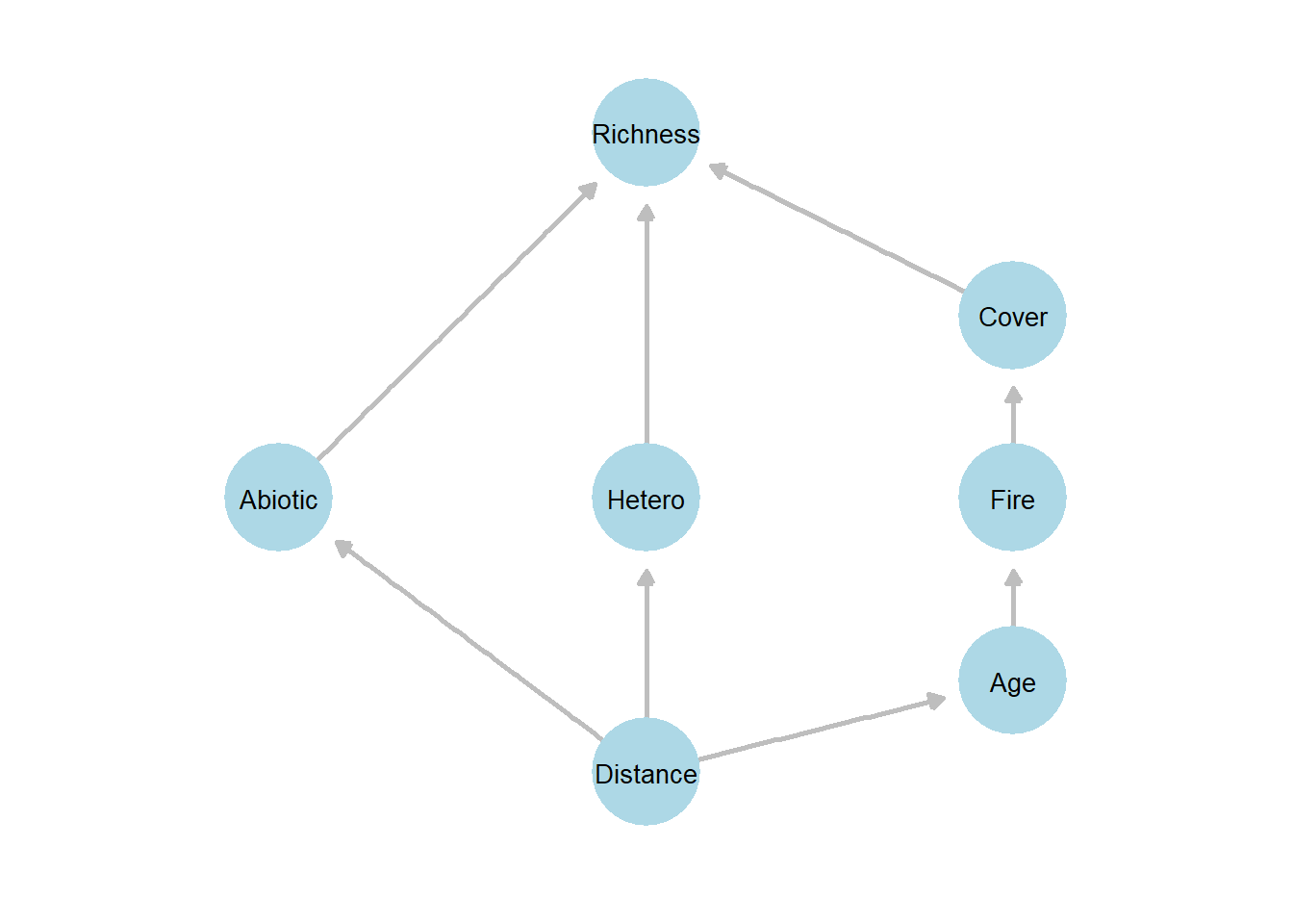
Figure 22.1: Conceptual path diagram illustrating the hypothesized relationships among landscape position, environmental conditions, disturbance, and plant diversity based on Grace and Keeley (2006). Arrows indicate directional (causal) paths specified in the piecewise structural equation model. Distance represents landscape position, which influences abiotic conditions, heterogeneity, and stand age. Fire severity and vegetation cover act as intermediate variables affecting plant species richness. The diagram represents the directed acyclic graph (DAG) used to define the component models in the piecewise SEM analysis.
The psem() function takes multiple “piecewise” model objects as input and combines them into a single causal network. From these component models, it constructs a path diagram and evaluates the implied conditional independence claims that define the structural equation model.
The conditional independence claims correspond to the missing paths in the proposed DAG. If any of these implied independence relationships are statistically violated —- meaning a missing path is in fact significant – this suggests that the proposed model structure is incomplete and may be omitting important biological relationships.
For this example, we begin by fitting a piecewise SEM in which all response variables are assumed to follow normal distributions. This reflects the original approach used by Grace and Keeley (2006) and provides a useful baseline for understanding how the method operates before extending it to more complex, non-normal models.
# Define individual models
m1 <- lm(abiotic ~ distance, data = df_keeley)
m2 <- lm(hetero ~ distance, data = df_keeley)
m3 <- lm(firesev ~ age, data = df_keeley)
m4 <- lm(cover ~ firesev, data = df_keeley)
m5 <- lm(rich ~ cover + abiotic + hetero, data = df_keeley)

# Combine into piecewise SEM
sem_model <- psem(m1, m2, m3, m4, m5)

# Evaluate
summary(sem_model, .progressBar = FALSE)
##
## Structural Equation Model of sem_model
##
## Call:
## abiotic ~ distance
## hetero ~ distance
## firesev ~ age
## cover ~ firesev
## rich ~ cover + abiotic + hetero
##
## AIC
## 1523.060
##
## ---
## Tests of directed separation:
##
## Independ.Claim Test.Type DF Crit.Value P.Value
## firesev ~ distance + ... coef 87 -1.6793 0.0967
## cover ~ distance + ... coef 87 1.3302 0.1869
## rich ~ distance + ... coef 85 3.1710 0.0021 **
## abiotic ~ age + ... coef 87 -0.0652 0.9481
## hetero ~ age + ... coef 87 0.0043 0.9966
## cover ~ age + ... coef 87 -1.8018 0.0750
## rich ~ age + ... coef 85 -1.2670 0.2086
## hetero ~ abiotic + ... coef 87 1.3296 0.1871
## firesev ~ abiotic + ... coef 86 -0.9713 0.3341
## cover ~ abiotic + ... coef 86 -0.2678 0.7895
## firesev ~ hetero + ... coef 86 0.4923 0.6237
## cover ~ hetero + ... coef 86 -2.7229 0.0078 **
## rich ~ firesev + ... coef 84 -1.3692 0.1746
##
## --
## Global goodness-of-fit:
##
## Chi-Squared = 30.929 with P-value = 0.003 and on 13 degrees of freedom
## Fisher's C = 48.924 with P-value = 0.004 and on 26 degrees of freedom
##
## ---
## Coefficients:
##
## Response Predictor Estimate Std.Error DF Crit.Value P.Value Std.Estimate
## abiotic distance 0.3998 0.0823 88 4.8562 0e+00 0.4597 ***
## hetero distance 0.0045 0.0013 88 3.4593 8e-04 0.3460 ***
## firesev age 0.0597 0.0125 88 4.7781 0e+00 0.4539 ***
## cover firesev -0.0839 0.0184 88 -4.5594 0e+00 -0.4371 ***
## rich cover 17.0138 3.7923 86 4.4864 0e+00 0.3573 ***
## rich abiotic 0.6847 0.1607 86 4.2609 1e-04 0.3481 ***
## rich hetero 55.3686 10.8212 86 5.1167 0e+00 0.4209 ***
##
## Signif. codes: 0 '***' 0.001 '**' 0.01 '*' 0.05
##
## ---
## Individual R-squared:
##
## Response method R.squared
## abiotic none 0.21
## hetero none 0.12
## firesev none 0.21
## cover none 0.19
## rich none 0.49Tests of directed separation: report which missing paths in the DAG are statistically significant. If any of these independence claims are rejected, it suggests that the proposed model structure may be incomplete. In this example, the relationships rich ~ distance + ... and cover ~ hetero + ... are identified as significant, indicating that these pathways may need to be explicitly included in the final model.
Global goodness-of-fit: reports both the chi-squared statistic and Fisher’s C. Unlike covariance-based SEM (e.g., lavaan), the chi-squared statistic in piecewise SEM is not derived from a variance–covariance matrix. Instead, it is computed by comparing the summed log-likelihoods of the component models under the saturated and unsaturated model structures, allowing the framework to accommodate non-normal response distributions.
Fisher’s C provides an alternative measure of overall model fit and is calculated as \(C = -2 \sum_i \ln(p_i)\), where \(i\) indexes each conditional independence claim and \(p_i\) is the corresponding p-value. Large values of Fisher’s C (i.e., small p-values) indicate that one or more independence assumptions are violated, suggesting that the proposed model may be missing important pathways.
Coefficients: summarizes the estimated effects for each component model. As in the lavaan framework, both raw parameter estimates (Estimate) and standardized coefficients (Std.Estimate) are reported. The raw estimates depend on the scale of the predictors and are therefore not directly comparable, whereas standardized estimates allow comparison of effect sizes across variables. Because this table clearly identifies the response and predictor variables for each path, it provides a concise and interpretable summary of the overall model output.
22.1.2 Post-fire plant diversity: the revised model
Because some of the response variables may be better described by non-normal distributions, we can extend the piecewise SEM framework by fitting generalized linear models. In particular, species richness is a count variable and is more appropriately modeled using a negative binomial distribution.
In addition, the analysis above highlighted potentially important pathways that were not included in the original DAG – specifically, the direct effects of landscape position (distance) on richness (rich) and heterogeneity (hetero) on vegetation cover (cover). These paths represent direct influences of each factor that may not be fully captured by the mediating variables in the original model.
Below, we revise the previous model by fitting species richness with a negative binomial GLM and adding missing paths.
# Define individual models
m1 <- lm(abiotic ~ distance, data = df_keeley)      # unchanged
m2 <- lm(hetero ~ distance, data = df_keeley)       # unchanged
m3 <- lm(firesev ~ age, data = df_keeley)           # unchanged

# m4 now includes a direct effect of hetero on cover (added path)
m4 <- lm(cover ~ firesev + hetero, data = df_keeley)

# m5 now models richness as negative binomial (MASS::glm.nb)
# and includes direct effect of distance on richness (added path)
m5 <- MASS::glm.nb(rich ~ cover + abiotic + hetero + distance,
                   data = df_keeley)

# Combine into piecewise SEM
sem_model <- psem(m1, m2, m3, m4, m5)

# Evaluate model
summary(sem_model, .progressBar = FALSE)
##
## Structural Equation Model of sem_model
##
## Call:
## abiotic ~ distance
## hetero ~ distance
## firesev ~ age
## cover ~ firesev + hetero
## rich ~ cover + abiotic + hetero + distance
##
## AIC
## 1514.731
##
## ---
## Tests of directed separation:
##
## Independ.Claim Test.Type DF Crit.Value P.Value
## firesev ~ distance + ... coef 87 -1.6793 0.0967
## cover ~ distance + ... coef 86 2.2342 0.0281 *
## abiotic ~ age + ... coef 87 -0.0652 0.9481
## hetero ~ age + ... coef 87 0.0043 0.9966
## rich ~ age + ... coef 84 -0.8843 0.3765
## cover ~ age + ... coef 86 -2.0164 0.0469 *
## hetero ~ abiotic + ... coef 87 1.3296 0.1871
## firesev ~ abiotic + ... coef 86 -0.9713 0.3341
## cover ~ abiotic + ... coef 85 0.1213 0.9038
## firesev ~ hetero + ... coef 86 0.4923 0.6237
## rich ~ firesev + ... coef 83 -1.5271 0.1267
##
## --
## Global goodness-of-fit:
##
## Chi-Squared = 17.339 with P-value = 0.098 and on 11 degrees of freedom
## Fisher's C = 30.829 with P-value = 0.1 and on 22 degrees of freedom
##
## ---
## Coefficients:
##
## Response Predictor Estimate Std.Error DF Crit.Value P.Value Std.Estimate
## abiotic distance 0.3998 0.0823 88 4.8562 0.0000 0.4597 ***
## hetero distance 0.0045 0.0013 88 3.4593 0.0008 0.3460 ***
## firesev age 0.0597 0.0125 88 4.7781 0.0000 0.4539 ***
## cover firesev -0.0859 0.0181 87 -4.7399 0.0000 -0.4472 ***
## cover hetero -0.5299 0.2607 87 -2.0329 0.0451 -0.1918 *
## rich cover 0.3277 0.0777 85 4.2200 0.0000 0.3102 ***
## rich abiotic 0.0096 0.0033 85 2.8888 0.0039 0.2206 **
## rich hetero 0.9762 0.2285 85 4.2718 0.0000 0.3344 ***
## rich distance 0.0103 0.0032 85 3.2787 0.0010 0.2725 **
##
## Signif. codes: 0 '***' 0.001 '**' 0.01 '*' 0.05
##
## ---
## Individual R-squared:
##
## Response method R.squared
## abiotic none 0.21
## hetero none 0.12
## firesev none 0.21
## cover none 0.23
## rich nagelkerke 0.78After including the previously missing paths, the Fisher’s C statistic became non-significant, indicating that the revised model fits the data reasonably well. The results can be visualized using the plot() function, where solid arrows indicate statistically significant pathways and dashed arrows indicate non-significant pathways.
plot(sem_model)
Figure 22.2: Visualization of the piecewise structural equation model for the Keeley dataset. Solid arrows indicate statistically significant pathways, while dashed arrows represent non-significant pathways. Node labels correspond to variables in the DAG: distance (distance to the coast), abiotic (abiotic conditions), hetero (habitat heterogeneity), age (stand age), firesev (fire severity), cover (vegetation cover), and rich (plant species richness).
22.2 Random Effects
22.2.1 Tree growth: data structure
Another simplifying assumption in traditional SEMs is that all data points are independent. This assumption is often violated, particularly when there are repeated measurements of the same individuals over time or when sampling is spatially clustered within a confined locality. Such hierarchical structures in the data-generating process should be properly accounted for. Piecewise SEM can accommodate this by incorporating random effects, allowing the model to account for non-independence among observations. We will use shipley data from Shipley 2009 to illustrate this case.
This dataset contains information on tree growth (Growth) and survival (Live) for a given observation year, along with environmental variables that may influence these demographic responses. These include cumulative degree days until first bud burst (DD) and the date of the first bud burst (Date).
Before proceeding with the analysis, we first perform data cleaning to ensure accuracy and consistency.
data("shipley")

df_shipley <- shipley %>%
  as_tibble() %>%
  janitor::clean_names() %>%
  drop_na(growth)
Importantly, this dataset contains temporally and spatially repeated measurements – the same individuals are tracked for growth over time until they die (tree indexes individuals), and five individuals are sampled at each site (site indexes locations). Clearly, these observations are not independent, and this hierarchical structure must be accounted for in the analysis.
df_shipley %>%
  group_by(site) %>%
  summarize(n_tree = n_distinct(tree))
## # A tibble: 20 × 2
## site n_tree
## <int> <int>
## 1 1 5
## 2 2 5
## 3 3 5
## 4 4 5
## 5 5 5
## 6 6 5
## 7 7 5
## 8 8 5
## 9 9 5
## 10 10 5
## 11 11 5
## 12 12 5
## 13 13 5
## 14 14 5
## 15 15 5
## 16 16 5
## 17 17 5
## 18 18 5
## 19 19 5
## 20 20 5To begin developing hypotheses, we first explore pairwise relationships among the variables.
# Pairwise plots of key variables
df_shipley %>%
  ggpairs(
    columns = c("dd",
                "date",
                "growth",
                "live"),  # select variables to plot
    progress = FALSE      # disable progress bar
  ) +
  theme_bw()              # clean theme for the plot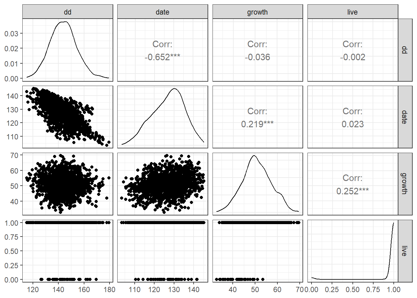
The relationships appear clear. Increasing cumulative degree days (dd) promotes earlier bud burst in trees (date; julian date of the year), which in turn may enhance both growth (growth) and survival (live).
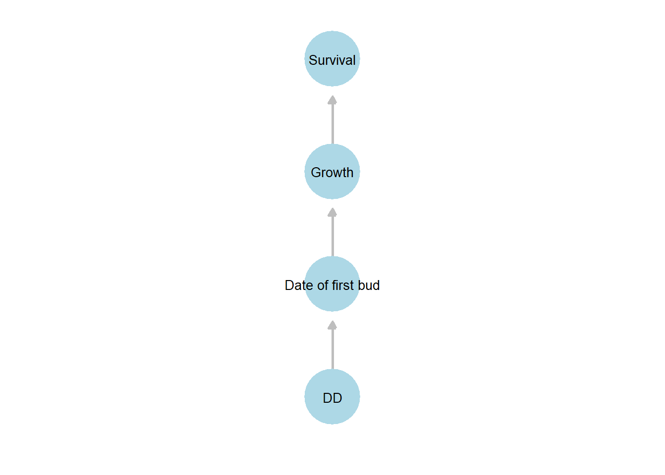
Figure 22.3: Directed acyclic graph (DAG) illustrating hypothesized relationships among the key variables in the shipley dataset. Arrows indicate the direction of hypothesized influence: cumulative degree days (DD) affects the date of first bud burst (Date of first bud), which influences Growth, and in turn affects Survival.
22.2.2 Tree growth: implementation
The psem() function accepts GLMMs of class glmmTMB or lmerMod (from the lme4 package), making it straightforward to include random effects in a piecewise SEM. In this example, we include site and tree as random effects. Since these are independent, unnested random effects, specifying them as separate terms in the model formula is appropriate.
# Model 1: date depends on dd, with random intercepts for site and tree
m1 <- glmmTMB(date ~ dd + (1 | site) + (1 | tree),
              data = df_shipley,
              family = "gaussian")

# Model 2: growth depends on date, same random effects
m2 <- glmmTMB(growth ~ date + (1 | site) + (1 | tree),
              data = df_shipley,
              family = "gaussian")

# Model 3: live (binary) depends on growth, logistic mixed model
m3 <- glmmTMB(live ~ growth + (1 | site) + (1 | tree),
              data = df_shipley,
              family = "binomial")

# Combine models into a piecewise SEM
sem_glmm <- psem(m1, m2, m3)

# Summarize SEM (paths, significance, and Shipley's test)
summary(sem_glmm, .progressBar = FALSE)
##
## Structural Equation Model of sem_glmm
##
## Call:
## date ~ dd
## growth ~ date
## live ~ growth
##
## AIC
## 12567.398
##
## ---
## Tests of directed separation:
##
## Independ.Claim Test.Type DF Crit.Value P.Value
## growth ~ dd + ... coef 1431 -0.2368 0.8128
## live ~ dd + ... coef 1431 -0.2234 0.8232
## live ~ date + ... coef 1431 -1.3764 0.1687
##
## --
## Global goodness-of-fit:
##
## Chi-Squared = 2.14 with P-value = 0.544 and on 3 degrees of freedom
## Fisher's C = 4.363 with P-value = 0.628 and on 6 degrees of freedom
##
## ---
## Coefficients:
##
## Response Predictor Estimate Std.Error DF Crit.Value P.Value Std.Estimate
## date dd -0.4976 0.0049 1431 -100.9187 0 -0.6281 ***
## growth date 0.3005 0.0268 1431 11.2202 0 0.3822 ***
## live growth 0.3479 0.0584 1431 5.9598 0 0.7866 ***
##
## Signif. codes: 0 '***' 0.001 '**' 0.01 '*' 0.05
##
## ---
## Individual R-squared:
##
## Response method Marginal Conditional
## date none 0.42 0.98
## growth none 0.11 0.83
## live none 0.56 0.63The model specification and interpretation are largely the same as before. In this case, both the chi-squared test and Fisher’s C were non-significant, indicating that the model fits the data well.
One key difference is the Individual R-squared: section, which now reports Marginal and Conditional values. These represent the model’s ability to explain variation using fixed effects only (marginal) or using both fixed and random effects (conditional). Because random effects often explain a substantial portion of the variation—particularly in the growth model—the conditional R-squared values are typically much higher. Note that these R-squared values are defined following Nakagawa and Schielzeth (2012) and differ from traditional R-squared.
22.3 Limitations
While piecewise SEM greatly expands the scope of data analysis, a notable limitation is the inability to incorporate latent variables—this feature is not implemented in the current package. However, the inclusion of latent variables is not a mathematical limitation, only a limitation of the implementation. Incorporating latent variables is possible within more generalized SEM frameworks, although the fitting process becomes more challenging. For those interested in this approach, Bayesian modeling offers a flexible alternative, and emerging packages (e.g., the brms package) increasingly allow such analyses without directly writing Stan or BUGS code. Nevertheless, these extensions require a solid understanding of the underlying statistical principles.