21 Structural Equation Modeling
In path analysis and structural equation modeling (SEM), we are interested in understanding the relationships among multiple variables simultaneously. Unlike simple regression, which models a single response as a function of one or more predictors, SEM allows researchers to specify networks of mediating pathways, providing a framework to quantify both direct and indirect contributions.
Learning Objectives:
Understand the conceptual difference between univariate regression, path analysis, and SEM.
Specify and fit path/SEM models using biological data, identifying direct and indirect effects.
Interpret model outputs, including path coefficients, residual variances, and fit statistics.
pacman::p_load(tidyverse,
               GGally,
               vegan,
               lavaan,
               lavaanPlot)
21.1 Path analysis
Path analysis is a special case of SEM. It is designed for cases where all variables of interest are directly measured, and you are interested in direct and indirect effects between those observed variables.
Let’s use the following data set, which involves plant, herbivore, and predator variables measured in 100 plots.
# Specify the URL of the raw CSV file on GitHub
url <- "https://raw.githubusercontent.com/aterui/biostats/master/data_raw/data_foodweb.csv"

# Read the CSV file into a tibble
(df_fw <- read_csv(url))
## # A tibble: 100 × 5
## plot_id mass_plant cv_h_plant mass_herbiv mass_pred
## <dbl> <dbl> <dbl> <dbl> <dbl>
## 1 1 99.3 4.98 50.3 24.6
## 2 2 99.8 4.97 49.9 24.7
## 3 3 102. 4.99 50.5 25.1
## 4 4 100. 4.96 50.2 24.9
## 5 5 100. 4.99 50.4 25.2
## 6 6 102. 5.05 50.4 25.1
## 7 7 100. 4.92 50.4 25.3
## 8 8 98.6 4.99 50.4 25.3
## 9 9 99.3 5.06 50.1 24.7
## 10 10 99.7 5.07 49.5 24.9
## # ℹ 90 more rowsThis dataset contains measurements for each plot, including plant biomass (mass_plant), variation in plant height expressed as the coefficient of variation (cv_h_plant), herbivore biomass (mass_herbiv), and predator biomass (mass_pred), along with a plot identifier (plot_id).
21.1.1 Directed acyclic graph
Given the bottom-up influences in this system, these variables may be sequentially connected, with plant biomass affecting herbivore biomass, which in turn affects predator biomass. At the same time, variation in plant height (cv_h_plant) may reflect shelter availability for herbivores, suggesting that this variable could also influence higher trophic levels.
In such a system, we can start with a full network represented as a directed acyclic graph (DAG), which encodes the hypothesized causal relationships among variables.
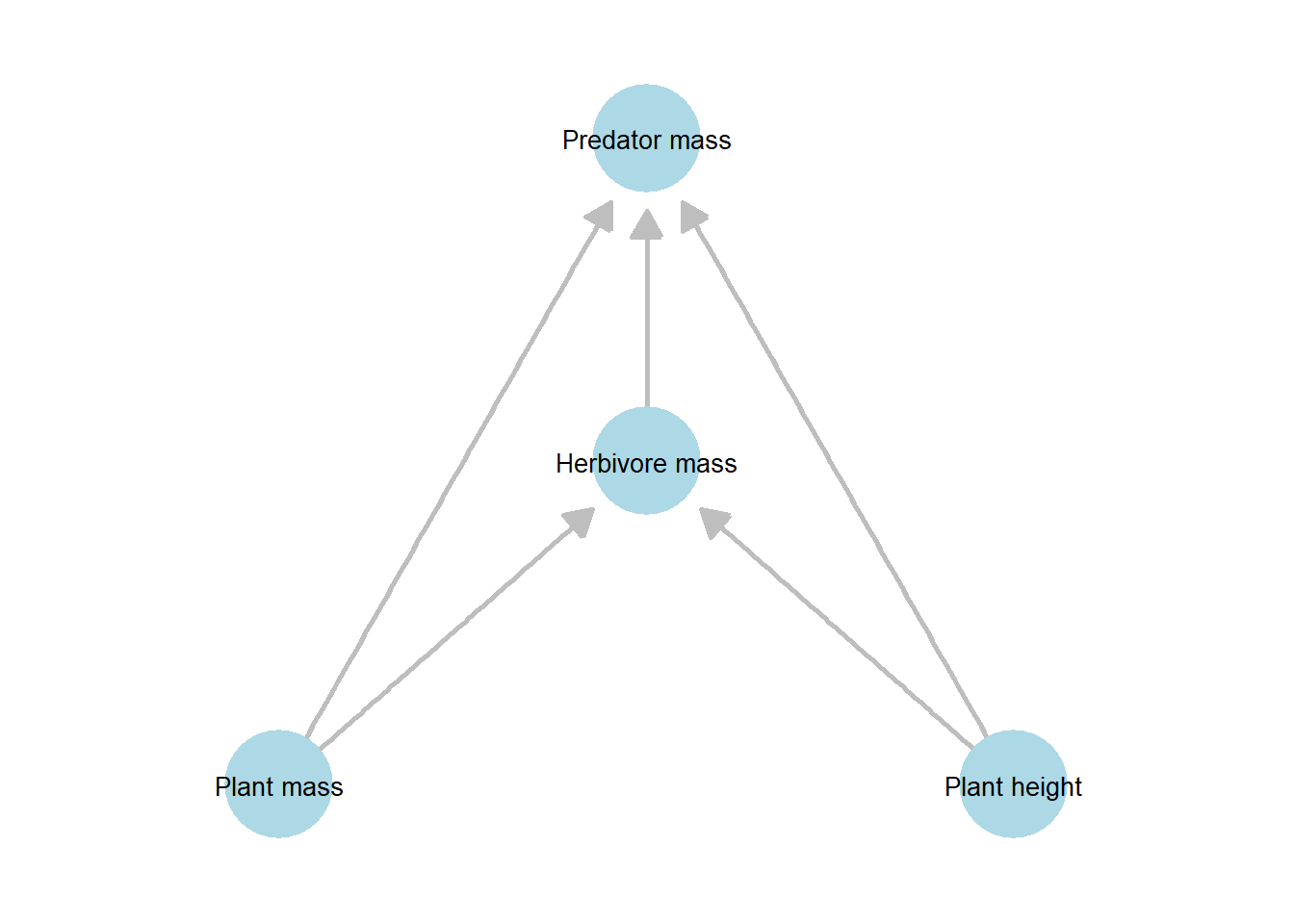
Figure 21.1: Directed acyclic graph (DAG) representing the hypothesized causal structure among plant, herbivore, and predator variables. Nodes denote measured variables (plant mass, plant height, herbivore mass, and predator mass), and directed edges indicate assumed directional effects. Plant mass and plant height are modeled as exogenous variables influencing herbivore mass, which in turn influences predator mass; plant variables may also have direct effects on higher trophic levels.
In these networks, discerning two types of variables is particularly important: endogenous and exogenous variables.
Endogenous variables are those whose values are influenced by other variables in the system; they have one or more incoming arrows in the DAG. In our example, herbivore and predator biomass are endogenous because they depend on plant biomass and other factors.
Exogenous variables are determined outside the system and are not influenced by other variables in the network; they only have outgoing arrows. For instance, plant biomass and variation in plant height can be treated as exogenous, as they drive changes in higher trophic levels without being influenced by them.
What makes this network a DAG is the absence of loops: all arrows flow from lower to higher trophic levels, with no feedback to lower levels. This excludes potential influences of higher trophic levels on lower ones (i.e., feedback loops). However, such cyclic relationships cannot be incorporated within the standard SEM framework, which is one of its major limitations.
21.1.2 Develop a hypothesis
The example above represents a full DAG, which serves as a reasonable starting point.
However, some links may not be biologically meaningful—for instance, while it is reasonable to assume that herbivore biomass is influenced by plant attributes, these variables are likely less important for predators.
Visualizing the network helps identify which links are potentially relevant among these variables.
df_fw %>%
  select(-plot_id) %>%        # remove plot_id column for plotting
  ggpairs(                    # create pairwise scatterplots and correlations
    progress = FALSE          # suppress progress messages
  ) +
  theme_bw()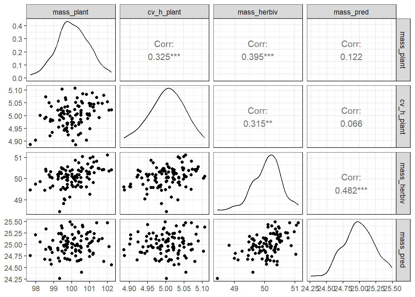
Plant variables are moderately correlated with herbivore biomass, not with predator biomass. These raw observations can guide hypothesis development and provide a rationale for omitting direct plant-to-predator paths from the DAG.
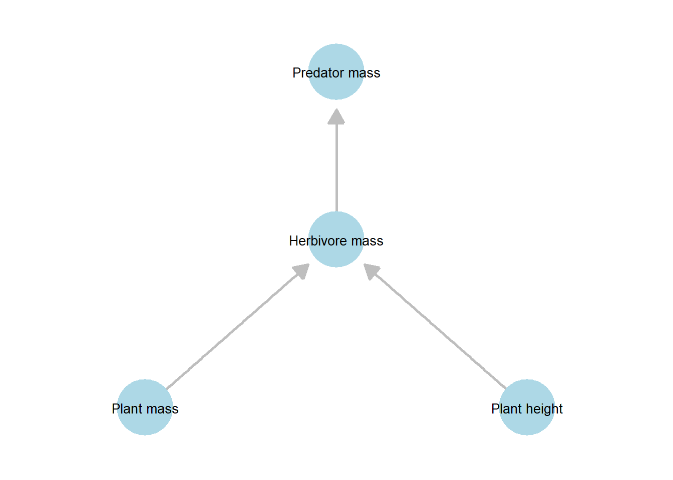
Figure 21.2: Simplified directed acyclic graph (DAG) representing the hypothesized causal relationships among plant, herbivore, and predator traits used in the focal analysis. Compared to the full DAG, this hypothesis-driven DAG retains only the direct pathways of primary interest, omitting direct links from plant variables to predator mass.
21.1.3 Implementation
A variety of R packages can be used to implement SEM, but here we will focus on lavaan, one of the most widely used packages for this purpose. A full description of its functionality is available on the lavaan website, but we will cover the basics here.
The key syntax is ~, which is used to specify a regression-like relationship between variables. Let’s start with a simple example. We first define a model that corresponds to our hypothetical DAG.
# Specify the SEM model using lavaan syntax
# Note: the variable names must exactly match the column names in the dataframe (df_fw)
m1 <- '
  # regression of herbivore biomass on plant variables
  mass_herbiv ~ mass_plant + cv_h_plant
  # regression of predator biomass on herbivore biomass
  mass_pred ~ mass_herbiv
'
The model description m1 should be passed to the sem() function from the lavaan package, which performs the analysis using the data you provide.
(fit1 <- sem(model = m1,
             data = df_fw))
## lavaan 0.6-12 ended normally after 1 iterations
##
## Estimator ML
## Optimization method NLMINB
## Number of model parameters 5
##
## Number of observations 100
##
## Model Test User Model:
##
## Test statistic 1.466
## Degrees of freedom 2
## P-value (Chi-square) 0.480The most important output from the sem() function is the Model Test User Model section, which reports the chi-square test statistic, degrees of freedom, and p-value.
The test statistic (1.466) measures the discrepancy between the SEM model-implied covariance matrix and the observed covariance matrix, while the degrees of freedom provide a sense of how simple the model is relative to the full DAG—that is, how many potential links from the full DAG are omitted. In other words, the test essentially asks: “Does the model adequately reproduce the observed relationships in the data?”
Unlike ordinary hypothesis tests, the p-value here tests the null hypothesis that the model fits the data perfectly. A high p-value (typically > 0.05) indicates no evidence of misfit. In this case, the p-value of 0.480 suggests that the model provides a good fit to the data.
We can obtain estimates for each path in the model, which quantify the strength of the relationships among variables:
summary(fit1, standardize = TRUE)## lavaan 0.6-12 ended normally after 1 iterations
##
## Estimator ML
## Optimization method NLMINB
## Number of model parameters 5
##
## Number of observations 100
##
## Model Test User Model:
##
## Test statistic 1.466
## Degrees of freedom 2
## P-value (Chi-square) 0.480
##
## Parameter Estimates:
##
## Standard errors Standard
## Information Expected
## Information saturated (h1) model Structured
##
## Regressions:
## Estimate Std.Err z-value P(>|z|) Std.lv Std.all
## mass_herbiv ~
## mass_plant 0.173 0.050 3.449 0.001 0.173 0.327
## cv_h_plant 2.052 0.935 2.195 0.028 2.052 0.208
## mass_pred ~
## mass_herbiv 0.244 0.044 5.497 0.000 0.244 0.482
##
## Variances:
## Estimate Std.Err z-value P(>|z|) Std.lv Std.all
## .mass_herbiv 0.185 0.026 7.071 0.000 0.185 0.805
## .mass_pred 0.045 0.006 7.071 0.000 0.045 0.768The Regressions: section is the most informative. The Estimate column reports the raw effect sizes, but these values depend on the units and variability of the predictor variables and therefore are not directly comparable across predictors.
By setting standardize = TRUE, however, lavaan also reports Std.all, which gives standardized coefficients (i.e., effects on a common scale). These standardized values allow direct comparison of the relative strength of different paths.
In this example, the strongest path is from mass_herbiv to mass_pred (0.482), followed by mass_plant to mass_herbiv (0.327), and cv_h_plant to mass_herbiv (0.208).
The results can be visualized with the lavaanPlot() function from lavaanPlot package.
lavaanPlot(model = fit1, coefs = TRUE, stand = TRUE)21.1.4 Model comparison
Our model omits all direct plant-to-predator pathways. However, variation in plant height may still influence predators indirectly by altering physical habitat structure. This possibility is represented in the following DAGs.
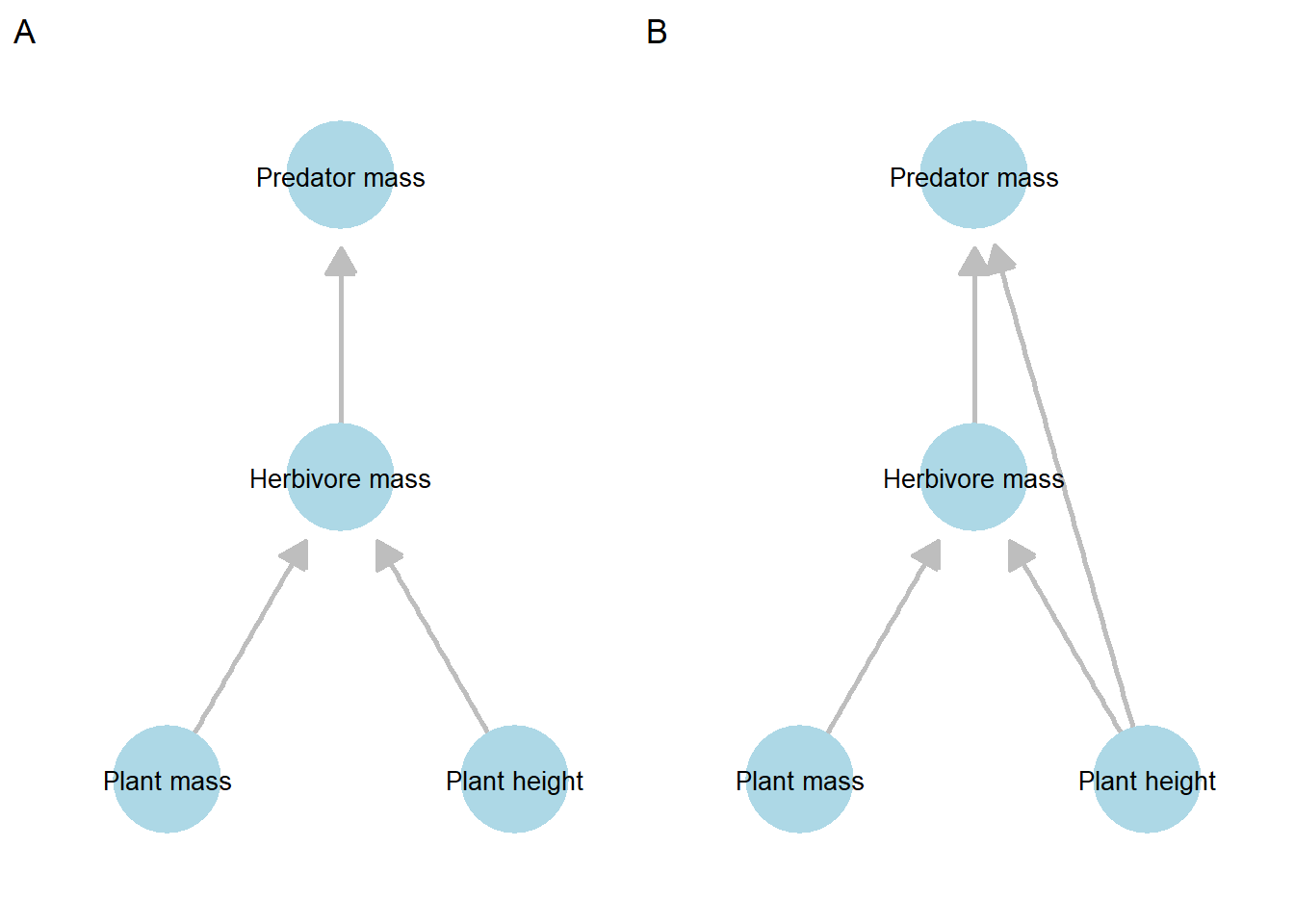
Figure 21.3: Comparison of two alternative directed acyclic graphs (DAGs) representing competing causal hypotheses among plant, herbivore, and predator variables. Panel A shows the hypothesized DAG, in which predator mass is influenced only indirectly through herbivore mass. Panel B shows an alternative DAG that includes an additional direct pathway from plant height to predator mass, representing a plausible but untested mechanism (e.g., habitat structure or plant-mediated effects).
How do we test this alternative hypothesis, and determine whether this new path is worth including?
We can address this by comparing model performance using a likelihood ratio test (LRT), which uses the difference in chi-square values between two models as the test statistic. The rationale is that the simpler model is a special case of the more complex model (i.e., the models are nested), so any improvement in fit can be attributed to the additional path.
If adding the new path substantially reduces the chi-square value relative to the increase in model complexity (degrees of freedom), this suggests that the path explains meaningful structure in the data and is worth including.
To perform this test, we first need to specify an alternative model that represents the updated DAG with the additional pathway:
m2 <- '
  mass_herbiv ~ mass_plant + cv_h_plant
  mass_pred ~ mass_herbiv + cv_h_plant
'

(fit2 <- sem(m2,
             data = df_fw))
## lavaan 0.6-12 ended normally after 1 iterations
##
## Estimator ML
## Optimization method NLMINB
## Number of model parameters 6
##
## Number of observations 100
##
## Model Test User Model:
##
## Test statistic 0.398
## Degrees of freedom 1
## P-value (Chi-square) 0.528We can use anova() function for the comparison.
anova(fit1, fit2)## Chi-Squared Difference Test
##
## Df AIC BIC Chisq Chisq diff Df diff Pr(>Chisq)
## fit2 1 99.826 115.46 0.3983
## fit1 2 98.894 111.92 1.4662 1.0678 1 0.3014This output shows a chi-square difference test comparing two nested SEMs. Here, fit2 is the more complex model with one fewer degree of freedom (Df = 1), and fit1 is the simpler model (Df = 2). Adding the extra path reduces the chi-square value from 1.4662 to 0.3983, giving a chi-square difference of 1.0678 with 1 degree of freedom.
The associated p-value (0.3014) is not significant, indicating that the more complex model does not provide a meaningful improvement in fit. Consistent with this result, information criteria (AIC and BIC) are slightly lower for fit1, supporting the conclusion that the simpler, more parsimonious model is preferred.
21.2 Structural Equation Modeling
In this section, we will extend a path analysis to structural equation modeling (SEM). What distinguishes a SEM from a simple path model is the ability to incorporate latent variables in the DAG.
Latent variables are “unobserved” variables that exist only within the statistical model. They are typically composites of multiple observed variables, often those that are strongly correlated with each other, and represent underlying constructs that cannot be measured directly.
21.2.1 SEM vs. Path analysis
To explore this, we will use the following dataset.
url <- "https://raw.githubusercontent.com/aterui/biostats/master/data_raw/data_herbivory.csv"

(df_herbv <- read_csv(url))
## # A tibble: 100 × 5
## soil_n herbivory sla cn_ratio per_lignin
## <dbl> <dbl> <dbl> <dbl> <dbl>
## 1 7.9 94.3 101. 9.4 6.9
## 2 10.5 97.7 100. 9.1 6.9
## 3 9.4 116. 99.9 9.7 8.1
## 4 9.1 101. 99.9 9.8 8
## 5 7.7 101. 99.4 10.6 8.1
## 6 10 117. 100. 9.4 7.8
## 7 8.2 105. 98.8 10.3 8.3
## 8 5.9 87.4 98.9 11.1 8.7
## 9 8.8 93.1 101 9.4 7.4
## 10 12.3 95.5 101. 10 7.8
## # ℹ 90 more rowsMeasurements were taken for individual plants grown under different levels of soil fertility, recorded in the column soil_n (inorganic nitrogen). These measurements are associated with each plant’s herbivory rate (herbivory), specific leaf area (sla), carbon-to-nitrogen ratio (cn_ratio), and percent lignin (per_lignin). The last three measurements – specific leaf area (sla), carbon-to-nitrogen ratio (cn_ratio), and percent lignin (per_lignin) – are plant traits that may affect herbivory rate.
At first glance, we might propose the following DAG, which models each plant trait and herbivory rate as separate, individual elements.
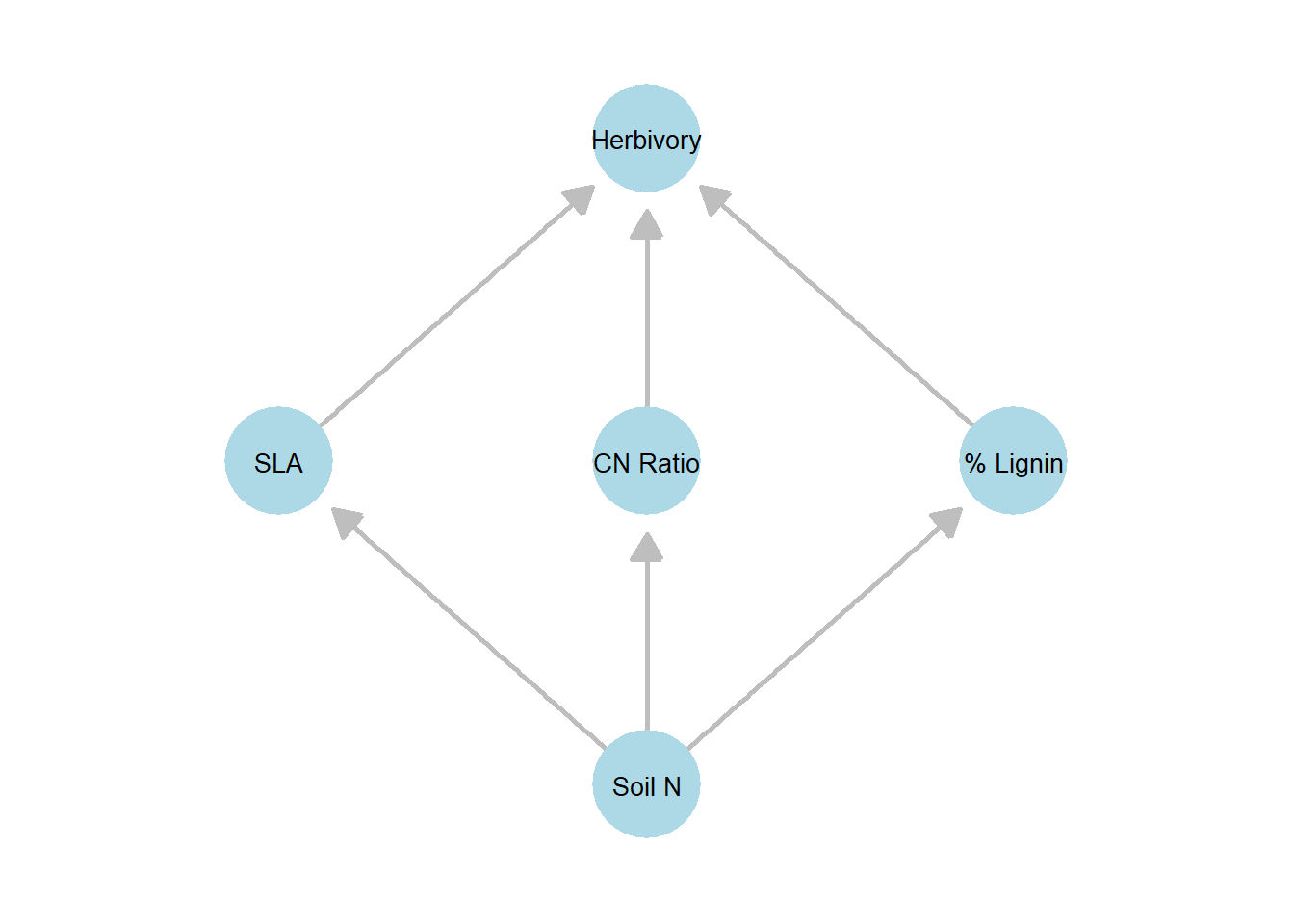
However, examining the three traits, we see that they are highly correlated and appear to be strongly influenced by soil inorganic nitrogen:
df_herbv %>%
  ggpairs(
    progress = FALSE,
    columns = c("soil_n",
                "sla",
                "cn_ratio",
                "per_lignin")
  ) +
  theme_bw()
These plant traits may collectively represent plant tissue “palatability,” which is influenced by soil fertility and, in turn, affects herbivory rate.
In this context, we can define a latent variable, palatability, as a function of the three plant traits. This latent variable then serves as a mediator linking soil fertility to herbivory rate. With this addition, the corresponding path diagram is modified to reflect the inclusion of the latent construct.
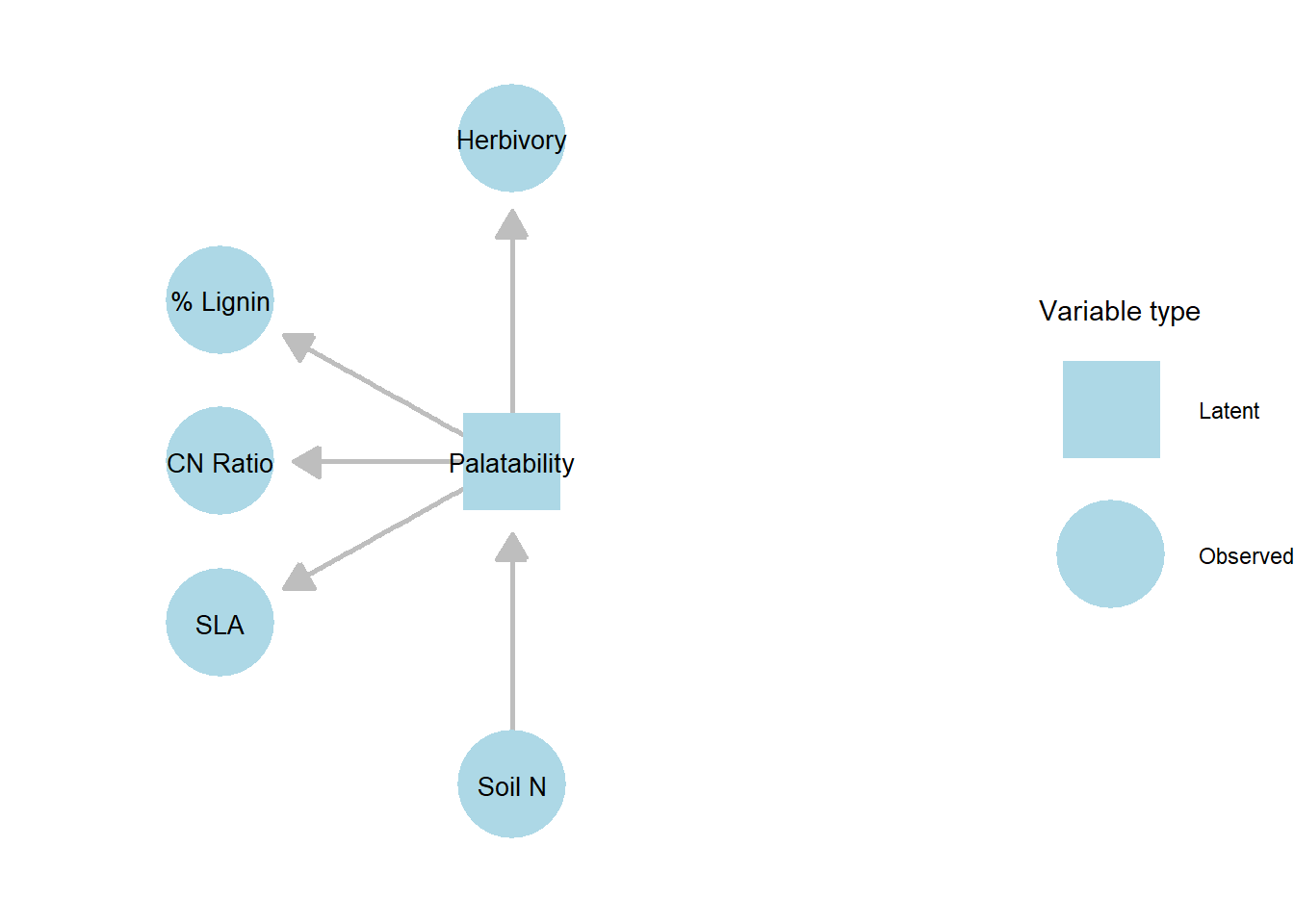
Figure 21.4: DAG of the structural equation model (SEM) linking soil fertility, palatability, and herbivory. Observed variables (SLA, CN Ratio, % Lignin, Soil N, Herbivory) are shown as circles, while the latent variable Palatability is shown as a square. Unlike a simple path analysis, SEM allows the inclusion of latent constructs that are inferred from multiple observed indicators, enabling the decomposition of complex traits like palatability into their underlying components.
21.2.2 Implementation
When implementing SEM, we use the special syntax =~ to specify latent variables in the model. In our example, we may use the following syntax: palatability =~ sla + cn_ratio + perlignin to construct a latent variable composed of three plant traits. By including latent constructs, SEM extends traditional path analysis, offering a more flexible framework to model complex relationships.
m_sem <- '
# latent variable
  palatability =~ sla + cn_ratio + per_lignin

# regression
  palatability ~ soil_n
  herbivory ~ palatability
'

(fit_sem <- sem(m_sem,
                data = df_herbv))
## lavaan 0.6-12 ended normally after 29 iterations
##
## Estimator ML
## Optimization method NLMINB
## Number of model parameters 9
##
## Number of observations 100
##
## Model Test User Model:
##
## Test statistic 8.970
## Degrees of freedom 5
## P-value (Chi-square) 0.110The primary output and its interpretation is similar - in this case, the p-value is > 0.05, suggesting that our model specification is reasonably good. We can exploit more information by calling summary():
summary(fit_sem, standardize = TRUE)## lavaan 0.6-12 ended normally after 29 iterations
##
## Estimator ML
## Optimization method NLMINB
## Number of model parameters 9
##
## Number of observations 100
##
## Model Test User Model:
##
## Test statistic 8.970
## Degrees of freedom 5
## P-value (Chi-square) 0.110
##
## Parameter Estimates:
##
## Standard errors Standard
## Information Expected
## Information saturated (h1) model Structured
##
## Latent Variables:
## Estimate Std.Err z-value P(>|z|) Std.lv Std.all
## palatability =~
## sla 1.000 0.616 0.884
## cn_ratio -0.837 0.067 -12.584 0.000 -0.516 -0.882
## per_lignin -1.107 0.079 -14.002 0.000 -0.682 -0.942
##
## Regressions:
## Estimate Std.Err z-value P(>|z|) Std.lv Std.all
## palatability ~
## soil_n 0.108 0.025 4.365 0.000 0.176 0.422
## herbivory ~
## palatability 4.190 1.480 2.832 0.005 2.581 0.284
##
## Variances:
## Estimate Std.Err z-value P(>|z|) Std.lv Std.all
## .sla 0.106 0.021 5.117 0.000 0.106 0.218
## .cn_ratio 0.076 0.015 5.162 0.000 0.076 0.221
## .per_lignin 0.059 0.019 3.080 0.002 0.059 0.112
## .herbivory 75.957 10.804 7.030 0.000 75.957 0.919
## .palatability 0.312 0.057 5.494 0.000 0.822 0.822The major difference from a simple path analysis is the inclusion of Latent Variables:, which decomposes the construct of palatability—a variable that exists only in the statistical model, not directly observed. The Estimate column shows the factor loadings, which indicate how strongly each observed variable contributes to the latent variable palatability.
In this example, palatability is positively associated with sla but negatively associated with cn_ratio and per_lignin. This means that higher palatability corresponds to leaves with higher specific leaf area (SLA), lower carbon-to-nitrogen ratio (C:N), and lower lignin content (% lignin).
The Regressions: section shows that the pathways from soil fertility to palatability and from palatability to herbivory rate are all significant, with the strongest effect observed between soil fertility and palatability.
21.3 Limitation
The examples above rely on one major assumption: in the lavaan package, all variables in the model are assumed to follow a normal distribution. This can be a restrictive assumption, especially given the variety of data types often encountered in biological research.
Importantly, this limitation comes from the package, not from the underlying statistics. Mathematically, it is possible to construct path analysis or SEM with non-normal variables or even include random effects.
However, such models are challenging to estimate using standard methods because the likelihood function becomes highly complex. In these cases, piecewise SEM (Lefcheck 2015) or Bayesian methods would provide a more flexible framework (examples: Takagi et al. 2014; Terui et al 2018). While there are currently few packages that allow fully automated implementation, coding models directly in BUGS or Stan makes it possible to fit these more complex SEMs (with a steep learning curve).